4Classical Machine Learning 4.5Classical Machine Learning Models
4.5.6 Decision Trees
Predict by following a sequence of simple feature-threshold questions from the root of a tree to a leaf.
What decision trees do
A decision tree predicts by asking a sequence of simple yes-or-no questions about individual features.
For an Iris flower, a tree might begin with:
Is petal width at most 0.8 cm?
→ yes: predict setosa
→ no: ask another question
The general process is:
sample → threshold question → left or right branch
       → another question → … → leaf → prediction
Trees can predict classes or numbers. A classification tree ends with a class such as setosa or virginica. A regression tree ends with a numeric value such as a house price.
This is different from the earlier models:
linear and logistic regression → combine all features in one weighted expression
K-NN                           → compare distances to stored examples
decision tree                  → inspect one feature at a time through repeated splits
The parts of a tree
A tree of depth 1 has one question and two leaves. It is often called a decision stump. More generally, a tree of depth can have at most leaves and internal nodes.
The following depth-2 tree is fitted to all 150 Iris flowers so that we can inspect its rules:
from sklearn.datasets import load_iris
from sklearn.tree import DecisionTreeClassifier, plot_tree
import matplotlib.pyplot as plt

iris = load_iris()
X, y = iris.data, iris.target

clf = DecisionTreeClassifier(max_depth=2, random_state=0)
clf.fit(X, y)

fig, ax = plt.subplots(figsize=(8, 4))
plot_tree(
    clf,
    feature_names=iris.feature_names,
    class_names=iris.target_names,
    filled=True,
    rounded=True,
    fontsize=10,
    ax=ax,
)
plt.show()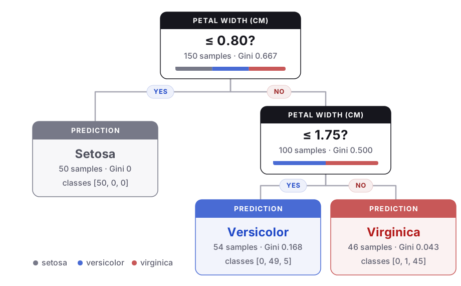
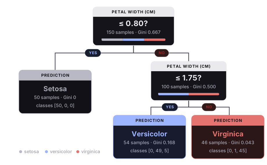
The root asks whether petal width is at most 0.80 cm. The left leaf predicts setosa. The right side asks another question at 1.75 cm, then predicts versicolor or virginica. This small tree uses only one of the four Iris features and classifies 144 of the 150 flowers correctly.
Following one prediction
Iris sample 150 has a petal width of 1.8 cm.
Question 1: Is 1.8 ≤ 0.80?
No → go right

Question 2: Is 1.8 ≤ 1.75?
No → go right

Leaf: virginica
A tree prediction is simply a path from the root to a leaf.
x_new = X[149:150]  # [5.9, 3.0, 5.1, 1.8]
print(clf.predict(x_new))
print(clf.predict_proba(x_new).round(3))
# [2]
# [[0.    0.022 0.978]]
For classification, predict_proba returns the class proportions among the training samples in the reached leaf. This leaf contains 1 versicolor and 45 virginica flowers, so its probabilities are and .
A prediction makes one comparison per level, so its cost is proportional to the tree's depth.
Using DecisionTreeClassifier in practice
For evaluation, split the labelled data before fitting:
from sklearn.model_selection import train_test_split
from sklearn.tree import export_text

X_train, X_test, y_train, y_test = train_test_split(
    X, y, test_size=0.2, stratify=y, random_state=0
)

model = DecisionTreeClassifier(max_depth=3, random_state=0)
model.fit(X_train, y_train)

predictions = model.predict(X_test)
probabilities = model.predict_proba(X_test)

print(round(model.score(X_test, y_test), 3))
print(export_text(model, feature_names=list(iris.feature_names)))
The most useful methods are:
fitlearns the questions from the training data;predictreturns the final class;predict_probareturns the class proportions in the reached leaf;scorereturns accuracy for a classifier;export_textprints the learned rules; andplot_treedraws the full structure.
Trees generally do not need StandardScaler. Their questions depend on whether a value is above or below a threshold, not on distances between feature values.
Why trees are useful
Decision trees are useful because they:
- handle non-linear relationships;
- discover interactions between features through successive questions;
- usually need no feature scaling;
- can be inspected and explained; and
- provide a quick baseline for tabular data.
The contrast with K-NN is especially helpful:
K-NN uses distances      → feature scale changes who is nearby
decision trees use order → scaling usually leaves the same splits
How a tree learns its questions
At each node, the tree follows the same process:
try possible feature-threshold questions
→ measure how well each question separates the labels
→ keep the best question
→ split the samples into two children
→ repeat separately in each child
This recursive procedure is called CART, short for Classification and Regression Trees. Breiman, Friedman, Olshen and Stone introduced it in their 1984 book of the same name.
Scikit-learn's DecisionTreeClassifier and DecisionTreeRegressor implement an optimised form of CART. CART always creates two branches. This differs from older methods such as ID3, which can build multiway trees; unlike C4.5, CART also handles numeric regression targets.
What makes one split better than another?
Suppose a node contains 50 red and 50 blue samples. It is very mixed.
A poor split might produce:
left:  25 red, 25 blue
right: 25 red, 25 blue
Both children are just as mixed as the parent, so the question has taught us nothing.
A useful split might produce:
left:  45 red,  5 blue
right:  5 red, 45 blue
Now each child is mostly one class. A good split makes the child nodes purer.
Gini impurity
Scikit-learn's default measure for classification is Gini impurity:
where is the fraction of samples belonging to class .
- If every sample has the same class, Gini impurity is 0: the node is pure.
- With two equally common classes, Gini impurity is : the node is highly mixed.
- Smaller Gini impurity means a purer node.
Another interpretation is that Gini impurity is the probability that two samples drawn at random, with replacement, have different labels.
Comparing the children
A split creates two children, often of different sizes. Their impurities are therefore weighted by the number of samples they contain:
CART chooses the split with the lowest weighted child impurity. Equivalently, it chooses the largest impurity decrease:
For the 100 non-setosa Iris flowers, the parent contains 50 versicolor and 50 virginica flowers, so its Gini impurity is 0.5. Splitting at petal width gives:
| Node | Versicolor | Virginica | Gini impurity |
|---|---|---|---|
| Parent | 50 | 50 | 0.5000 |
| Left child | 49 | 5 | 0.1680 |
| Right child | 1 | 45 | 0.0425 |
The weighted child impurity is about 0.1103, so the impurity decrease is about . That large decrease makes this a strong split.
OptionalOptional mathematics: the full Iris Gini calculation
The parent impurity is
The left child has 54 samples:
The right child has 46 samples:
Weighting by child size gives
No other feature-threshold pair at this node produces a lower value. The best split on petal length reaches about 0.1265. These node impurities are available in clf.tree_.impurity.
OptionalOptional: entropy
Another impurity measure is entropy:
where a term with is treated as 0. Like Gini impurity, entropy is 0 for a pure node and larger for a more mixed node.
| Fraction of class 1 | 0 | 0.1 | 0.25 | 0.5 |
|---|---|---|---|---|
| Gini impurity | 0 | 0.180 | 0.375 | 0.500 |
| Entropy | 0 | 0.469 | 0.811 | 1.000 |
For three equally common classes, entropy is . Scikit-learn uses criterion="gini" by default; "entropy" and its synonym "log_loss" are alternatives. Gini and entropy often select similar splits, so Gini is a sensible starting point.
Which thresholds are tried?
For a numeric feature, CART sorts the distinct values at the current node and tries the midpoints between neighboring values.
For example, if the values are
one candidate threshold is the midpoint between 0.6 and 1.0:
The resulting question is “is this feature at most 0.8?” At the Iris root, petal width has 22 distinct values, so CART tries 21 thresholds for that feature. A setosa petal is at most 0.6 cm wide, while every other flower has width at least 1.0 cm, so the midpoint 0.8 separates setosa perfectly.
OptionalOptional: formal CART algorithm and why it is greedy
At a node , let be the samples that reach it. A candidate tests feature at threshold and creates left and right subsets. Its weighted impurity is
CART chooses and repeats the search inside each child.
function grow(samples, depth):
    if a stopping rule applies:
        return leaf(samples)

    for every feature:
        for every midpoint between neighboring values:
            calculate weighted child impurity
    keep the feature and threshold with the lowest impurity

    left = samples that pass the question
    right = all other samples
    return node(question, grow(left), grow(right))
The algorithm is greedy: it chooses the best split available now without testing every possible future tree. Finding a globally optimal tree is computationally difficult—NP-complete under several definitions of optimality—so practical algorithms use this shortcut. It can miss a weak-looking split that would enable excellent later splits; XOR and parity patterns are examples that greedy trees can find awkward.
Tree depth and overfitting
A shallow tree contains a few broad rules. It may miss important patterns and underfit. A deeper tree can describe smaller regions and fit the training data better. If it grows too deep, it can create tiny regions around individual samples and memorise noise.
The pattern to watch is:
training accuracy   → usually keeps increasing with depth
validation accuracy → may level off or fall
The Breast Cancer dataset contains 569 samples with 30 numeric features. The following code holds out 30% for validation and grows trees of increasing depth:
from sklearn.datasets import load_breast_cancer

cancer = load_breast_cancer()
X_train, X_val, y_train, y_val = train_test_split(
    cancer.data,
    cancer.target,
    test_size=0.3,
    stratify=cancer.target,
    random_state=0,
)

for depth in [1, 2, 3, 4, 5, 6, 8, None]:
    fitted = DecisionTreeClassifier(max_depth=depth, random_state=0)
    fitted.fit(X_train, y_train)
    print(depth, fitted.get_depth(), fitted.get_n_leaves(),
          f"{fitted.score(X_train, y_train):.3f}",
          f"{fitted.score(X_val, y_val):.3f}")
max_depth |
Depth reached | Leaves | Training accuracy | Validation accuracy |
|---|---|---|---|---|
| 1 | 1 | 2 | 0.932 | 0.889 |
| 2 | 2 | 4 | 0.942 | 0.906 |
| 3 | 3 | 8 | 0.980 | 0.901 |
| 4 | 4 | 12 | 0.990 | 0.906 |
| 5 | 5 | 15 | 0.997 | 0.912 |
| 6 | 6 | 16 | 1.000 | 0.906 |
| 8 | 6 | 16 | 1.000 | 0.906 |
None |
6 | 16 | 1.000 | 0.906 |
At depth 6 the training score reaches 1.000, but the validation score does not improve. The growing gap shows that later splits are fitting the training set rather than learning a reliable pattern.
One validation sample changes accuracy by about , so differences of one or two samples are not strong evidence. Cross-Validation gives a steadier comparison of depths. Never choose tree depth from training accuracy alone.
Controlling tree complexity
The three most useful controls for a first tree are:
| Setting | Default | Effect |
|---|---|---|
max_depth |
None |
Limits the number of levels |
min_samples_split |
2 |
Stops small nodes from splitting |
min_samples_leaf |
1 |
Prevents tiny leaves |
max_depth is usually the easiest place to start because its effect can be seen directly in the drawn tree. A float passed to either sample-count setting is interpreted as a fraction of the training set.
OptionalOptional: more tree-size controls and pruning
max_leaf_nodeslimits the total number of leaves. The tree grows best-first, expanding nodes with the largest relative impurity decrease.min_impurity_decreaseallows a split only when its weighted impurity decrease reaches a chosen minimum.max_featureslimits how many randomly selected features are considered at a split. This rarely helps a single tree but is central to Random Forests.ccp_alphacontrols cost-complexity pruning. This post-pruning method first grows a larger tree and then removes weak branches. The scikit-learn example Post pruning decision trees with cost complexity pruning follows the full pruning path.
The User Guide suggests max_depth=3 as a useful starting point for inspecting a tree and min_samples_leaf=5 as an initial leaf-size limit.
OptionalOptional: ties and random_state
Scikit-learn randomly permutes features at each split, even when all features are considered. If two splits have exactly the same impurity decrease, that order decides the winner.
At the Iris root, petal width and petal length both separate the 50 setosa flowers perfectly. With random_state=0, the depth-2 tree chooses petal width; with random_state=42, it chooses petal length. Set random_state to an integer when you need reproducible results.
Regression trees
The tree structure does not change for regression. A leaf simply predicts a number instead of a class. It usually predicts the mean target of the training samples in that leaf:
Splits try to make the numeric targets within each child similar. The default node impurity is their mean squared deviation from the node mean:
The parallel is:
classification → make class labels purer within each leaf
regression     → make numeric targets more similar within each leaf
The diabetes dataset records ten baseline measurements for 442 patients. This depth-2 tree uses BMI to predict disease progression one year later:
import numpy as np
from sklearn.datasets import load_diabetes
from sklearn.tree import DecisionTreeRegressor

diabetes = load_diabetes(scaled=False)
X_bmi = diabetes.data[:, [2]]
y_prog = diabetes.target

reg = DecisionTreeRegressor(max_depth=2, random_state=0)
reg.fit(X_bmi, y_prog)
print(export_text(reg, feature_names=["bmi"]))
print(reg.predict([[20.0], [24.0], [25.0], [30.0], [35.0]]).round(2))|--- bmi <= 27.25
| |--- bmi <= 24.35
| | |--- value: [105.04]
| |--- bmi > 24.35
| | |--- value: [143.96]
|--- bmi > 27.25
| |--- bmi <= 33.15
| | |--- value: [191.56]
| |--- bmi > 33.15
| | |--- value: [264.23]
[105.04 105.04 143.96 191.56 264.23]The four leaves contain 165, 112, 135 and 30 patients, and their predictions are the corresponding means: 105.04, 143.96, 191.56 and 264.23.
With one feature, a regression tree produces a step function: every input in one interval receives the same prediction. It also does not extrapolate naturally. A BMI larger than anything in the training data still receives the value of the last leaf rather than continuing an upward trend.
DecisionTreeRegressor also provides criterion="absolute_error", whose leaves predict medians, and criterion="poisson" for non-negative targets such as counts.
OptionalOptional mathematics: why a leaf predicts the mean
Suppose a leaf must use one constant prediction . Its squared error is
The derivative is
This equals zero when . The mean is therefore the constant with the smallest squared error, and the remaining mean squared error is the variance of the targets in the leaf.
How trees create non-linear rules
A tree does not assume a straight-line relationship. It can ask different questions in different parts of the feature space:
if x₁ ≤ 3:
    use one rule
else:
    if x₂ ≤ 7:
        use another rule
The effect of now depends on the earlier value of . This is an interaction. Linear and logistic regression often need an interaction feature such as to be added by hand; a tree can create the interaction through its path.
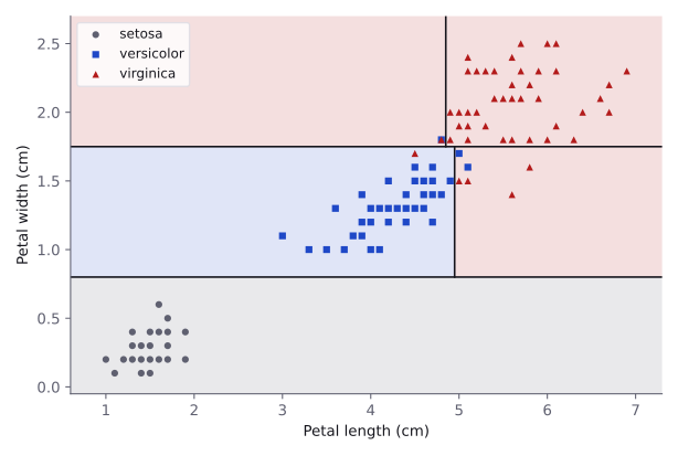
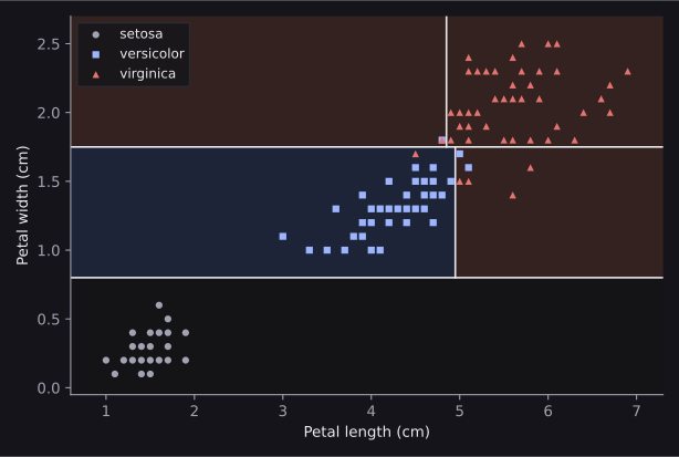
Each leaf also describes a rectangular region where one prediction is used. Together, the leaves make the tree a piecewise constant function.
Axis-aligned boundaries
Each question tests one feature, so a two-dimensional split is vertical or horizontal. A diagonal or curved boundary must be approximated by a staircase of rectangular regions.
rng = np.random.default_rng(0)
P = rng.uniform(size=(2000, 2))
labels = (P[:, 0] > P[:, 1]).astype(int)
P_train, P_test, l_train, l_test = train_test_split(
    P, labels, test_size=0.5, random_state=0
)

for depth in [1, 2, 4, 8]:
    fitted = DecisionTreeClassifier(max_depth=depth, random_state=0)
    fitted.fit(P_train, l_train)
    print(depth, fitted.get_n_leaves(),
round(fitted.score(P_test, l_test), 3))1 2 0.729
2 4 0.857
4 13 0.951
8 30 0.976Even with 30 leaves, the staircase still misclassifies 2.4% of the test points.
Feature engineering can still help
The true rule above is . If we create the feature
then the entire rule becomes , which a one-question tree can represent:
D_train = (P_train[:, 0] - P_train[:, 1]).reshape(-1, 1)
D_test = (P_test[:, 0] - P_test[:, 1]).reshape(-1, 1)

stump = DecisionTreeClassifier(max_depth=1, random_state=0)
stump.fit(D_train, l_train)
print(stump.score(D_test, l_test))  # 1.0
Trees automatically model many non-linear rules, but a useful engineered feature can still make an awkward rule dramatically simpler.
This creates a useful connection across models:
linear regression → features change what a weighted sum can represent
K-NN              → features change what “nearby” means
decision tree     → features change what simple thresholds can express
No feature scaling is usually needed
A tree depends on the ordering of feature values. Standardisation changes the values but keeps their order, so it usually divides the samples in exactly the same way and only changes the written thresholds.
On the Breast Cancer split above, trees fitted to the raw features, standardised features, and transformed features make identical predictions for all 171 validation samples.
Do not scale data automatically just because it is machine learning. Distance-based models such as K-NN need scaling; decision trees generally do not.
A single tree can be unstable
Small changes in the training data can change an early split. That changes which samples reach every node below it, so the rest of the tree—and some predictions—can also change.
When the unrestricted Breast Cancer tree was refitted on four random subsets containing 90% of the training data:
- the new trees had 11 to 14 leaves instead of 16;
- one of the four changed the root feature; and
- 11 to 14 of the 171 validation predictions changed.
This high variance is one of the largest weaknesses of a single tree. Random Forests fit many trees to varied samples and average their predictions to reduce the instability. XGBoost instead builds shallow trees in sequence, each correcting earlier errors.
Feature importances
Splits near the top of a tree often affect many samples. A feature receives importance when splits using it reduce impurity. Scikit-learn stores these scores in feature_importances_.
names = cancer.feature_names
full_tree = DecisionTreeClassifier(random_state=0)
full_tree.fit(X_train, y_train)

importance = full_tree.feature_importances_
for j in np.argsort(importance)[::-1][:3]:
    print(names[j], importance[j].round(3))
print((importance > 0).sum())worst perimeter 0.8
mean texture 0.066
worst concave points 0.042
11Only 11 of the 30 features are used. An importance of 0 does not prove that a feature is useless. Worst radius and worst area have correlations of 0.994 and 0.978 with worst perimeter; the tree can use worst perimeter and ignore the two features that carry almost the same information.
Impurity-based importance can also be misleading on an overfit tree and is biased towards features with many distinct values. Permutation importance measures how much a validation score falls when a feature is shuffled, which is often a better diagnostic.
OptionalOptional mathematics: exact impurity-based importance
The importance of feature is the sum of the weighted impurity decreases at nodes that use it:
is the number of training samples; , and are the counts at the node and its children; and denotes their impurities. The final importances are normalised to sum to 1. This is also called the mean decrease in impurity or MDI.
OptionalOptional: categorical features and missing values
Categorical features. The scikit-learn 1.9.1 User Guide states that its decision trees do not directly support categorical variables. Encode them first; OneHotEncoder is a common choice because a split can then separate one category from the others.
Missing values. With the default splitter="best", DecisionTreeClassifier and DecisionTreeRegressor accept NaN values in X. During fitting, each candidate split is evaluated with missing samples sent left and with them sent right. The better direction is stored and reused during prediction. Data Cleaning covers general missing-data strategies.
Useful decision-tree settings and methods
| Setting | Default | Meaning |
|---|---|---|
criterion |
"gini" for classification |
How split quality is measured |
splitter |
"best" |
How candidate thresholds are chosen |
class_weight |
None |
Class importance for classification |
random_state |
None |
Reproducibility of random choices |
A fitted tree also provides:
get_depth()andget_n_leaves()for its size;apply(X)for the leaf reached by each sample;decision_path(X)for the nodes each sample visits;cost_complexity_pruning_path(X,y)for pruning candidates; andtree_, whose arrays describe every node.
export_text has max_depth and decimals settings for controlling the printed rules. plot_tree draws each question, impurity, sample count, class counts and majority class.
Optional: finding one split from scratch
After sorting samples by one feature, cumulative class counts let us score every possible cut efficiently:
def gini(counts):
    p = counts / counts.sum(axis=1, keepdims=True)
    return 1.0 - (p ** 2).sum(axis=1)


def best_split_1d(x, y, n_classes):
    order = np.argsort(x)
    x, y = x[order], y[order]
    n = len(x)

    onehot = np.eye(n_classes)[y]
    left = np.cumsum(onehot, axis=0)[:-1]
    right = onehot.sum(axis=0) - left
    n_left = np.arange(1, n)

    weighted_gini = (
        n_left * gini(left) + (n - n_left) * gini(right)
    ) / n
    weighted_gini[x[1:] == x[:-1]] = np.inf

    i = np.argmin(weighted_gini)
    return weighted_gini[i], (x[i] + x[i + 1]) / 2


def best_split(X, y):
    n_classes = y.max() + 1
    results = [
        best_split_1d(X[:, j], y, n_classes) + (j,)
        for j in range(X.shape[1])
    ]
    weighted_gini, threshold, feature = min(results)
    return feature, threshold, weighted_gini


j, threshold, weighted_gini = best_split(X_train, y_train)
print(names[j], round(threshold, 4), round(weighted_gini, 4))
# worst perimeter 106.1 0.1236
Scikit-learn chooses the same root split: worst perimeter , with weighted child impurity 0.1236. The next-best feature, worst radius, reaches 0.1307, so this choice is not a tie. Sorting costs per feature, and CART repeats the search at every node.
Decision trees in olympiad tasks
A shallow tree is a fast, interpretable baseline for tabular data. export_text reveals which features and thresholds it uses. A tree can also be fixed by a task, leaving feature engineering as the only way to improve the result.
A depth-4 tree has at most 16 leaves and 15 questions, and any prediction follows at most four comparisons. The 1,496 raw values of one widget may contain global patterns, varying positions or summary information that four raw thresholds cannot express.
The effective pipeline was therefore:
raw 187 × 8 array → meaningful summary features → shallow decision treeThe organisers' baseline used the standard deviation across the eight columns at each of the 187 rows. It achieved validation ROC AUC of 0.639 at depth 20 and 0.604 at depth 4. The official best-solution notebook reports 0.973 and 0.945. At a high level, its features normalised each widget and reduced dependence on position along the 187 rows.
The lesson is the same one seen across this module: if a tree has only a few questions, each feature must expose useful structure in a form that a simple threshold can detect.
When should I try a decision tree?
A decision tree is a good choice when:
- the data is tabular;
- relationships are non-linear;
- feature interactions matter;
- an inspectable baseline is useful; or
- you do not want to scale numeric features.
Be cautious when:
- the tree grows very deep;
- the dataset is small or noisy;
- stable predictions are important; or
- the boundary is awkward for vertical and horizontal splits.
The whole idea in one view
prediction:      sample → threshold question → left or right
                 → repeat → leaf → prediction

training:        candidate feature-threshold splits → measure impurity
                 → choose the best split → repeat recursively

complexity:      shallow tree → simple rules → possible underfitting
                 deep tree → detailed rules → possible overfitting

classification:  leaf → class and class proportions
                 split quality → Gini impurity or entropy

regression:      leaf → mean target
                 split quality → squared error or variance

strengths:       no scaling → non-linear rules → interactions
                 → inspectable decisions

weaknesses:      deep trees overfit → axis-aligned boundaries
→ instability from small data changesResources
| Source | Title | Why read it |
|---|---|---|
| scikit-learn | User Guide: Decision Trees | Read 'Mathematical formulation' for the split criteria, 'Missing Values Support' for how NaN values are routed, and 'Minimal Cost-Complexity Pruning' for ccp_alpha. |
| scikit-learn | DecisionTreeClassifier | Every hyperparameter with its default, fitted attributes such as tree_ and feature_importances_, and methods such as cost_complexity_pruning_path. |
| scikit-learn | Post pruning decision trees with cost complexity pruning | Follows the pruning path of a tree on the breast cancer dataset and chooses ccp_alpha from validation scores. |
| Google for Developers | Decision Forests course: Decision trees | Short illustrated pages. 'Growing decision trees', 'Exact splitter for binary classification with numerical features' and 'Overfitting and pruning' follow this module closely. The code uses the YDF library, not scikit-learn. |
| James et al. | An Introduction to Statistical Learning with Python, section 8.1 | Free book. Section 8.1, 'The Basics of Decision Trees', covers regression trees, classification trees and cost-complexity pruning; section 8.2 continues with bagging, random forests and boosting. |
| StatQuest | Decision and Classification Trees, Clearly Explained!!! | Builds a classification tree step by step with Gini impurity, including numeric features and ways to prevent overfitting. |
Practice problems
| Solved | Source | Problem | Difficulty | Tags |
|---|---|---|---|---|
| IOAI 2024 | Save the Factory | Hard | tabular, feature engineering | |
| Kaggle | Titanic | Easy | tabular, categorical, missing values |
Finished this module? Mark it done.
Comments
Stuck on something, spotted a mistake, or found a resource that helped you? Tell us below.
Loading comments