4Classical Machine Learning 4.7Post-Training Theory
4.7.1 Model Evaluation Metrics
A practical framework for choosing, interpreting and implementing classification and regression metrics, including custom IOAI scores.
What does a metric do?
A model can be evaluated in several reasonable ways. A classifier may have high accuracy but miss most examples of a rare class. A regressor may have a small average error but still make a few very large mistakes. The metrics disagree because they care about different behaviour.
A metric turns a set of predictions and true answers into a number. In an IOAI task, that number determines the score, so the task's metric is part of the problem—not an afterthought.
Approaching a Typical Problem explains where evaluation fits into the workflow. This module focuses on how common metrics behave and how to compute them. Clustering metrics are introduced separately in K-Means Clustering.
Start with the model output
Different metrics expect different forms of output.
| Model output | What it contains | Common metrics |
|---|---|---|
| Class labels | One final class per sample | Accuracy, balanced accuracy, precision, recall, F1 |
| Scores | A value used to rank samples | ROC AUC, average precision |
| Probabilities | Confidence assigned to each class | Log loss |
| Numeric predictions | A number such as a price or count | MAE, MSE, RMSE, , MAPE |
The same classifier may provide all three classification outputs. Logistic regression, for example, produces probabilities; those probabilities can rank samples or be converted to labels with a threshold.
Four shared questions distinguish the metrics:
| Question | Why it matters |
|---|---|
| Is higher or lower better? | Accuracy is maximised; errors such as RMSE are minimised. |
| Do all samples or classes count equally? | Macro and group averages can stop large groups from dominating. |
| Does it use a threshold? | Label metrics change with the decision threshold; ranking metrics do not. |
| How are large mistakes treated? | Squared errors grow faster than absolute errors; log loss heavily punishes confident mistakes. |
Every metric card below uses the same fields: input, behaviour, direction, suitable uses, risks and scikit-learn name.
Metrics in IOAI tasks
IOAI tasks show why the exact definition matters.
| Task | Prediction | Metric | Better |
|---|---|---|---|
| Save the Factory (2024) | One of two classes | ROC AUC computed from predicted labels | Higher |
| Help BOBAI (2024, on-site) | One of seven classes | Macro F1 | Higher |
| Lost in Hyperspace (2024) | Three numeric properties | RMSE of each property, weighted by , and , then averaged | Lower |
| Antique Painting Authentication (2025) | One of two classes | Accuracy | Higher |
| Chicken Counting (2025) | A density map whose sum is the count | $\exp\bigl(-\frac{1}{n}\sum_i | y_i-\hat y_i |
| Synthetic Speech Detector (2025, GAITE) | One of two classes | Macro F1 | Higher |
| Robot Chasing (2026) | One of six actions | Accuracy for each robot, averaged on a 0–100 scale | Higher |
| Operation Night Watch (2026) | One of 29 classes | Half old-class clip accuracy plus half new-class clip accuracy | Higher |
Some tasks use one sklearn.metrics function. Others add weights, average groups or define a new formula. Save the Factory even passed labels—not probabilities—to roc_auc_score. Small details can change the meaning of the score.
The confusion matrix
Most label-based classification metrics come from one shared table. In binary classification, one class is called positive, usually the class we want to detect, and the other is negative.
| Outcome | Meaning |
|---|---|
| True positive (TP) | A positive sample predicted positive |
| False positive (FP) | A negative sample predicted positive |
| False negative (FN) | A positive sample predicted negative |
| True negative (TN) | A negative sample predicted negative |
The first word says whether the prediction was correct; the second says which class was predicted. For classes, entry of the confusion matrix counts samples of true class predicted as class . Correct predictions lie on the diagonal.
OptionalWorked example: build a confusion matrix
The examples use logistic regression with two Breast Cancer features. Malignant tumours are the positive class. Scikit-learn codes them as 0, so 1 - target recodes them as 1.
from sklearn.datasets import load_breast_cancer
from sklearn.linear_model import LogisticRegression
from sklearn.metrics import confusion_matrix
from sklearn.model_selection import train_test_split
from sklearn.pipeline import make_pipeline
from sklearn.preprocessing import StandardScaler

cancer = load_breast_cancer(as_frame=True)
X = cancer.data[["mean radius", "mean texture"]]
y = 1 - cancer.target
X_train, X_test, y_train, y_test = train_test_split(
    X, y, test_size=0.25, stratify=y, random_state=0
)
model = make_pipeline(StandardScaler(), LogisticRegression())
model.fit(X_train, y_train)
y_pred = model.predict(X_test)

print(confusion_matrix(y_test, y_pred))
# [[87  3]
#  [ 8 45]]
tn, fp, fn, tp = confusion_matrix(y_test, y_pred).ravel()| Predicted benign (0) | Predicted malignant (1) | |
|---|---|---|
| True benign (0) | TN = 87 | FP = 3 |
| True malignant (1) | FN = 8 | TP = 45 |
Scikit-learn puts true classes in rows and predicted classes in columns, both in sorted label order. For labels 0 and 1, ravel() returns TN, FP, FN and TP. Other sources sometimes put the positive class first.
The multiclass examples later use these predictions:
y3_true = [0, 0, 0, 0, 0, 1, 1, 1, 2, 2]
y3_pred = [0, 0, 0, 0, 0, 1, 1, 0, 2, 0]
print(confusion_matrix(y3_true, y3_pred))
# [[5 0 0]
#  [1 2 0]
#  [1 0 1]]
The labels argument fixes row and column order. ConfusionMatrixDisplay.from_predictions draws the matrix.
Accuracy and balanced accuracy
Accuracy
| Field | Accuracy |
|---|---|
| Input | Predicted labels |
| Formula | |
| Rewards | Correct predictions, with every sample weighted equally |
| Range | 0 to 1; higher is better |
| Use when | Classes have similar importance and no class overwhelms the data |
| Be careful when | A common class can hide failure on a rare class |
| scikit-learn | accuracy_score |
In the three-class example, accuracy is . An always-largest-class classifier can therefore look strong without learning the other classes.
Balanced accuracy
| Field | Balanced accuracy |
|---|---|
| Input | Predicted labels |
| Formula | , the mean recall over classes |
| Rewards | Doing well on every class, regardless of class size |
| Range | 0 to 1; higher is better |
| Use when | Classes are imbalanced but should matter equally |
| Be careful when | The task genuinely values samples rather than classes equally |
| scikit-learn | balanced_accuracy_score |
The class recalls in the example are , and , so balanced accuracy is . An always-one-class classifier has balanced accuracy .
from sklearn.metrics import accuracy_score, balanced_accuracy_score

print(round(accuracy_score(y_test, y_pred), 3))            # 0.923
print(round(balanced_accuracy_score(y_test, y_pred), 3))   # 0.908
print(accuracy_score(y3_true, y3_pred))                    # 0.800
print(round(balanced_accuracy_score(y3_true, y3_pred), 3)) # 0.722
Averaging accuracy over other groups
Balanced accuracy averages group accuracy over true classes. The same idea can use other groups.
- Robot Chasing averages accuracy over six robots. With 600 samples per robot, this equals ordinary accuracy.
- Operation Night Watch gives equal weight to the old-class and new-class groups, even though they contain different numbers of clips and classes.
import numpy as np

def mean_group_accuracy(y_true, y_pred, groups):
    """Accuracy inside each group, averaged with equal weights."""
    y_true, y_pred, groups = map(np.asarray, (y_true, y_pred, groups))
    scores = [np.mean(y_pred[groups == g] == y_true[groups == g])
              for g in np.unique(groups)]
    return float(np.mean(scores))

print(round(mean_group_accuracy(y3_true, y3_pred, y3_true), 3))  # 0.722
is_old = np.asarray(y3_true) < 2
print(mean_group_accuracy(y3_true, y3_pred, is_old))             # 0.6875
The old group has correct and the new group , giving .
Precision, recall and F1
These metrics focus on the positive class and ignore TN.
Precision
| Field | Precision |
|---|---|
| Formula | |
| Answers | Of the positive predictions, how many are correct? |
| Use when | False alarms are costly |
| Be careful when | Predicting very few positives can raise precision while missing most positives |
| scikit-learn | precision_score |
Recall
| Field | Recall |
|---|---|
| Formula | |
| Answers | Of the truly positive samples, how many were found? |
| Other names | Sensitivity; true positive rate (TPR) |
| Use when | Missing a positive is costly |
| Be careful when | Predicting nearly everything positive can raise recall while causing false alarms |
| scikit-learn | recall_score |
The negative class's recall, , is specificity or the true negative rate.
F1
| Field | F1 score |
|---|---|
| Formula | |
| Rewards | Precision and recall being high together |
| Range | 0 to 1; higher is better |
| Use when | Both missed positives and false alarms matter |
| Be careful when | It ignores TN and depends on the threshold |
| scikit-learn | f1_score |
For the tumour model, precision is , recall is , and F1 is .
from sklearn.metrics import f1_score, precision_score, recall_score

print(round(precision_score(y_test, y_pred), 3))  # 0.938
print(round(recall_score(y_test, y_pred), 3))     # 0.849
print(round(f1_score(y_test, y_pred), 3)) # 0.891OptionalWhy F1 uses the harmonic mean, and how F-beta changes it
The harmonic mean is pulled towards the smaller value. If only the tumour with the highest probability is labelled malignant, precision is perfect but recall is almost zero:
proba = model.predict_proba(X_test)[:, 1]
top1 = (proba == proba.max()).astype(int)
print(precision_score(y_test, top1))         # 1.000
print(round(recall_score(y_test, top1), 3))  # 0.019
print(round(f1_score(y_test, top1), 3))      # 0.037
The arithmetic mean would be 0.509 and hide the poor recall. When precision and recall should not count equally, use
favours recall and favours precision. For the tumour model they are 0.865 and 0.918 respectively.
If no sample is predicted positive, precision becomes . Scikit-learn returns 0 with an UndefinedMetricWarning; zero_division can set 0, 1 or np.nan. Recall is similarly undefined when the true positive class is absent. pos_label chooses the positive class; its default is 1.
Averaging over classes
For multiclass data, each class can be treated as positive in turn before the results are combined.
| Average | How it combines classes | Practical meaning |
|---|---|---|
| Macro | Unweighted mean | Every class matters equally |
| Weighted | Mean weighted by support | Large classes matter more |
| Micro | Add TP, FP and FN first | Every individual decision matters equally |
| Class | Precision | Recall | F1 | Support |
|---|---|---|---|---|
| 0 | 0.714 | 1.000 | 0.833 | 5 |
| 1 | 1.000 | 0.667 | 0.800 | 3 |
| 2 | 1.000 | 0.500 | 0.667 | 2 |
For this example, macro F1 is 0.767, weighted F1 is 0.790 and micro F1 is 0.800. In single-label classification, micro F1 equals accuracy. Macro recall equals balanced accuracy.
from sklearn.metrics import classification_report

print(classification_report(y3_true, y3_pred, digits=3))
for average in ["macro", "weighted", "micro"]:
    print(average, round(f1_score(y3_true, y3_pred,
                                  average=average), 3))
# macro 0.767
# weighted 0.790
# micro 0.800
Help BOBAI and Synthetic Speech Detector use macro F1, so small classes count as much as large ones. Synthetic Speech Detector averages the F1 of bonafide and spoof samples; this is not default binary F1. For the tumour example, class F1 values are [0.941, 0.891], giving macro F1 0.916 instead of positive-class F1 0.891.
Thresholds, ROC curves and AUC
Most classifiers first produce a score or probability. A decision threshold turns it into a label: predict positive when the score is at least .
Lower thresholds usually find more positives but also create more false alarms.
OptionalWorked example: moving the threshold
proba = model.predict_proba(X_test)[:, 1]
for t in [0.1, 0.3, 0.5, 0.7, 0.9]:
    pred_t = (proba >= t).astype(int)
    tn, fp, fn, tp = confusion_matrix(y_test, pred_t).ravel()
    print(f"t={t:.1f} TP={tp:2} FP={fp:2} "
          f"TPR={tp/(tp+fn):.3f} FPR={fp/(fp+tn):.3f}")
# t=0.1 TP=52 FP=34 TPR=0.981 FPR=0.378
# t=0.3 TP=48 FP= 7 TPR=0.906 FPR=0.078
# t=0.5 TP=45 FP= 3 TPR=0.849 FPR=0.033
# t=0.7 TP=39 FP= 1 TPR=0.736 FPR=0.011
# t=0.9 TP=32 FP= 0 TPR=0.604 FPR=0.000
Moving from 0.5 to 0.3 finds three more malignant tumours but adds four false alarms. Moving to 0.9 removes every false alarm but misses 21 malignant tumours.
ROC AUC
| Field | ROC AUC |
|---|---|
| Input | Scores or probabilities, normally before thresholding |
| Definition | Area under TPR versus FPR over all thresholds |
| Interpretation | Probability that a random positive outranks a random negative, with ties worth one half |
| Range | About 0.5 for uninformative scores; 1 for perfect ranking; higher is better |
| Use when | Comparing rankings across thresholds |
| Be careful when | Positives are rare, or the final threshold and probability quality matter |
| scikit-learn | roc_auc_score, roc_curve |
ROC AUC depends only on score order, so decision_function and probabilities give the same value when they preserve that order.
from sklearn.metrics import roc_auc_score

print(round(roc_auc_score(y_test, proba), 3)) # 0.970OptionalThe pairwise AUC formula
For every positive and negative ,
The tumour example contains positive-negative pairs:
pos = proba[y_test.to_numpy() == 1]
neg = proba[y_test.to_numpy() == 0]
diff = pos[:, None] - neg[None, :]
print(round(np.mean(diff > 0) + 0.5 * np.mean(diff == 0), 3)) # 0.970ROC AUC of hard labels
If roc_auc_score receives 0/1 labels instead of scores, its area is
which is exactly balanced accuracy.
print(round(roc_auc_score(y_test, y_pred), 4))            # 0.9079
print(round(balanced_accuracy_score(y_test, y_pred), 4))  # 0.9079
Save the Factory evaluated model.predict(...) with roc_auc_score, so its reported ROC AUC was balanced accuracy, as noted in Decision Trees.
Precision–recall curves and average precision
| Field | Average precision (AP) |
|---|---|
| Input | Scores or probabilities |
| Definition | Summary of the precision–recall curve over thresholds |
| Baseline | Roughly the fraction of positives for uninformative scores |
| Use when | The positive class is rare and positive predictions must remain useful |
| Be careful when | Comparing datasets with very different positive rates |
| scikit-learn | average_precision_score, precision_recall_curve |
ROC divides false positives by all negatives, so many false positives can look small when negatives are extremely common. The precision–recall curve makes that failure more visible.
OptionalWorked example: ROC AUC and AP with rare positives
from sklearn.datasets import make_classification
from sklearn.metrics import average_precision_score

X_r, y_r = make_classification(
    n_samples=6000, weights=[0.95], random_state=0
)
X_tr, X_rest, y_tr, y_rest = train_test_split(
    X_r, y_r, test_size=0.5, stratify=y_r, random_state=0
)
X_val, X_te, y_val, y_te = train_test_split(
    X_rest, y_rest, test_size=0.5, stratify=y_rest, random_state=0
)
clf = LogisticRegression().fit(X_tr, y_tr)
s_val = clf.predict_proba(X_val)[:, 1]
s_te = clf.predict_proba(X_te)[:, 1]

print(round(y_te.mean(), 3))                          # 0.054
print(round(roc_auc_score(y_te, s_te), 3))            # 0.914
print(round(average_precision_score(y_te, s_te), 3))  # 0.476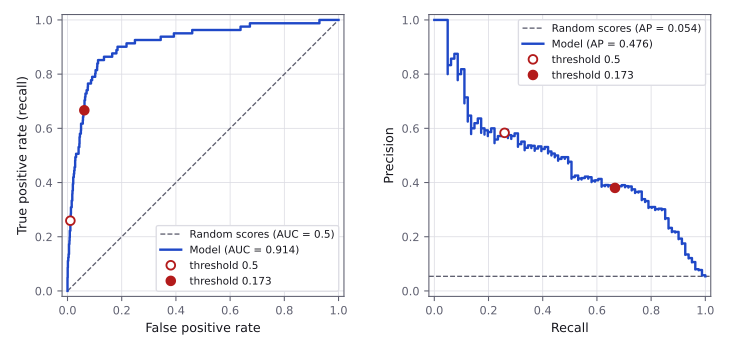
Average precision can be written as
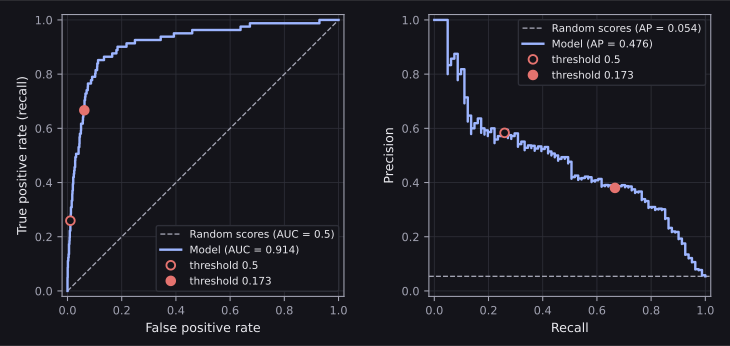
where thresholds run from high to low. Here AUC is 0.914 but AP is 0.476; at threshold 0.5, precision is 0.583 and recall only 0.259.
Choosing a threshold
A label metric such as F1 depends on the threshold. Choose it using validation data or cross-validation, never the test set.
from sklearn.metrics import precision_recall_curve

prec, rec, thr = precision_recall_curve(y_val, s_val)
f1 = 2 * prec * rec / np.maximum(prec + rec, 1e-12)
best = thr[np.argmax(f1[:-1])]
print(round(best, 3))  # 0.173
for t in [0.5, best]:
    print(round(f1_score(y_te, (s_te >= t).astype(int)), 3))
# 0.359
# 0.484
Threshold 0.173 raises test F1 from 0.359 to 0.484: recall rises from 0.259 to 0.667 while precision falls from 0.583 to 0.380. TunedThresholdClassifierCV performs this search with cross-validation.
Log loss
| Field | Log loss |
|---|---|
| Input | Predicted class probabilities |
| Formula | |
| Rewards | High probability on the true class and honest confidence |
| Range | 0 is perfect; lower is better; no finite upper bound |
| Use when | Probability quality matters, not only labels or ranking |
| Be careful when | A confidently wrong prediction receives a very large penalty |
| scikit-learn | log_loss |
Log loss works with any number of classes. It is also the training loss of logistic regression.
from sklearn.metrics import log_loss

y_ll = np.array([1] * 50 + [0] * 50)
p_ll = np.where(y_ll == 1, 0.9, 0.1)
print(round(log_loss(y_ll, p_ll), 3))  # 0.105
p_ll[0] = 0.001
print(round(log_loss(y_ll, p_ll), 3))  # 0.173
p_ll[0] = 0.0
print(round(log_loss(y_ll, p_ll), 3))  # 0.465
A true-class probability of exactly 0 would have infinite loss. Scikit-learn clips it near machine precision, about , producing a sample loss near 36. Never submit exact 0 or 1 probabilities for a log-loss task. Loss Functions compares log loss with other training losses.
Regression metrics
For residual , regression metrics differ mainly in how quickly the penalty grows and whether the scale of the label matters.
MAE, MSE and RMSE
| Metric | Formula | Units | Behaviour | scikit-learn |
|---|---|---|---|---|
| MAE | $\frac1n\sum_i | r_i | $ | Label units |
| MSE | Squared units | Large errors count disproportionately | mean_squared_error |
|
| RMSE | Label units | Same ranking as MSE, easier to interpret | root_mean_squared_error |
All are lower-is-better. Use MAE when a mistake twice as large should cost about twice as much. Use RMSE when occasional large mistakes deserve extra emphasis.
from sklearn.metrics import (mean_absolute_error, mean_squared_error,
                             root_mean_squared_error)

y_reg = np.array([50, 60, 70, 80, 90])
pred_a = np.array([52, 58, 72, 78, 92])
pred_b = np.array([52, 58, 72, 78, 110])
for pred in [pred_a, pred_b]:
    print(mean_absolute_error(y_reg, pred),
          mean_squared_error(y_reg, pred),
          round(root_mean_squared_error(y_reg, pred), 2))
# 2.0 4.0 2.0
# 5.6 83.2 9.12
Changing one error from 2 to 20 multiplies MAE by 2.8 but RMSE by 4.6.
The coefficient of determination
| Field | |
|---|---|
| Formula | |
| Interpretation | Squared error compared with predicting the evaluation labels' mean |
| Range | 1 is perfect, 0 matches that mean baseline, and values can be negative; higher is better |
| Use when | Comparing models on the same labels with a scale-free score |
| Be careful when | Scores from different evaluation sets or groups are not directly comparable |
| scikit-learn | r2_score; also the default .score() of regressors |
On one fixed set, and MSE rank models identically. can be negative on new data because the model does not know the test labels' mean.
OptionalWhy R-squared can be negative or change across groups
A constant model fitted to the diabetes training mean scores 0 on training data and slightly below 0 on test data because the means differ.
from sklearn.datasets import load_diabetes
from sklearn.dummy import DummyRegressor

Xd, yd = load_diabetes(return_X_y=True)
Xd_tr, Xd_te, yd_tr, yd_te = train_test_split(
    Xd, yd, test_size=0.2, random_state=0
)
mean_model = DummyRegressor(strategy="mean").fit(Xd_tr, yd_tr)
print(round(mean_model.score(Xd_tr, yd_tr), 3))  # 0.0000
print(round(mean_model.score(Xd_te, yd_te), 4))  # -0.0013
It also depends on label spread. A model predicting iris petal width has and RMSE 0.231 cm over all 45 test flowers. On 16 setosa flowers, RMSE improves to 0.132 cm but falls to −0.215 because their widths barely vary: variance is 0.0144 while model MSE is 0.0175.
from sklearn.datasets import load_iris
from sklearn.linear_model import LinearRegression
from sklearn.metrics import r2_score

iris = load_iris(as_frame=True).frame
X_i = iris[["petal length (cm)"]]
y_i = iris["petal width (cm)"]
X_itr, X_ite, y_itr, y_ite = train_test_split(
    X_i, y_i, test_size=0.3, random_state=0
)
reg = LinearRegression().fit(X_itr, y_itr)
w_pred = reg.predict(X_ite)
print(round(r2_score(y_ite, w_pred), 3),
      round(root_mean_squared_error(y_ite, w_pred), 3))  # 0.896 0.231

setosa = (iris.loc[X_ite.index, "target"] == 0).to_numpy()
print(round(r2_score(y_ite[setosa], w_pred[setosa]), 3),
      round(root_mean_squared_error(y_ite[setosa],
                                    w_pred[setosa]), 3))  # -0.215 0.132
The overfit degree-3 example in Linear Regression is another negative- case.
Relative errors
| Field | MAPE / mean relative absolute error |
|---|---|
| Formula | $\frac1n\sum_i |
| Rewards | Small error relative to each label's size |
| Range | 0 is perfect; lower is better |
| Use when | A fixed absolute error should matter more for small labels |
| Be careful when | Labels can be zero or close to zero; over- and underprediction are not fully symmetric |
| scikit-learn | mean_absolute_percentage_error, returned as a fraction |
Chicken Counting uses , so its score is higher when relative error is lower.
from sklearn.metrics import mean_absolute_percentage_error

def chicken_score(y_true, y_pred):
    y_true, y_pred = np.asarray(y_true), np.asarray(y_pred)
    relative_error = np.abs(y_true - y_pred) / y_true
    return float(np.exp(-np.mean(relative_error)))

counts = np.array([40, 25, 10])
pred_counts = np.array([36, 27, 13])
mape = mean_absolute_percentage_error(counts, pred_counts)
print(round(mape, 3), round(chicken_score(counts, pred_counts), 3))
# 0.160 0.852
The error of 3 on 10 counts three times as much as the error of 4 on 40. Predicting 0 can undercount by at most 100%, but overcounting is unbounded: predicting 30 instead of 10 gives relative error 2.
Choosing a metric
Use the task statement first. When designing an evaluation, this flow gives a starting point.
Classification
├─ Final labels matter
│  ├─ Classes have similar size and importance → accuracy
│  ├─ Every class should count equally → balanced accuracy or macro F1
│  ├─ False positives matter most → precision
│  ├─ False negatives matter most → recall
│  └─ Need one balance of precision and recall → F1 or F-beta
├─ Ranking across thresholds matters → ROC AUC
├─ Positives are rare and their quality matters → average precision
└─ Probability quality matters → log loss

Regression
├─ Typical absolute error matters → MAE
├─ Large errors deserve extra punishment → RMSE
├─ Need performance relative to label variation → R²
└─ Error relative to target size matters → MAPE or a task formula
No metric is universally best. The right one is the metric whose rewards and penalties match the task.
Metrics in scikit-learn
| Metric | Function in sklearn.metrics |
Input | Better |
|---|---|---|---|
| Accuracy, balanced accuracy | accuracy_score, balanced_accuracy_score |
Labels | Higher |
| Precision, recall, F1, | precision_score, recall_score, f1_score, fbeta_score |
Labels | Higher |
| Confusion matrix, report | confusion_matrix, classification_report |
Labels | — |
| ROC AUC, ROC curve | roc_auc_score, roc_curve |
Scores | Higher |
| Average precision, precision–recall curve | average_precision_score, precision_recall_curve |
Scores | Higher |
| Log loss | log_loss |
Probabilities | Lower |
| MAE, MSE, RMSE, MAPE | mean_absolute_error, mean_squared_error, root_mean_squared_error, mean_absolute_percentage_error |
Numbers | Lower |
r2_score |
Numbers | Higher |
Metric functions take true values first: f1_score(y_true, y_pred). Swapping the arguments of precision_score, for example, computes recall instead.
Scoring strings
Cross-validation and tuning tools accept metric names through scoring. A scorer such as "roc_auc" calls predict_proba or decision_function itself.
from sklearn.model_selection import cross_val_score

for scoring in ["accuracy", "f1_macro", "roc_auc", "neg_log_loss"]:
    scores = cross_val_score(model, X_train, y_train, cv=5,
                             scoring=scoring)
    print(f"{scoring:13}{scores.mean():.3f}")
# accuracy      0.878
# f1_macro      0.866
# roc_auc       0.947
# neg_log_loss -0.279
Scorers always treat larger values as better. Scikit-learn therefore negates errors: "neg_log_loss" is minus log loss and "neg_root_mean_squared_error" is minus RMSE. The best value is closest to zero. sklearn.metrics.get_scorer_names() lists every string.
Custom metrics
make_scorer adapts a function of (y_true, y_pred) for cross-validation. Set greater_is_better=False for an error, or response_method="predict_proba" when the function needs probabilities.
from sklearn.metrics import make_scorer

chicken_scorer = make_scorer(chicken_score)
scores = cross_val_score(LinearRegression(), X_itr, y_itr, cv=5,
                         scoring=chicken_scorer)
print(scores.round(3))  # [0.890 0.809 0.841 0.782 0.785]
The scorer can be passed to Hyperparameter Tuning and Cross-Validation. When a metric needs extra information such as robot IDs, it can be clearer to predict on validation data and call mean_group_accuracy directly.
The whole idea in one view
task goal
   ↓
choose what the metric should reward
   ↓
match the metric to the model output
labels → accuracy, balanced accuracy, precision, recall, F1
scores → ROC AUC, average precision
probabilities → log loss
numbers → MAE, RMSE, R², relative error
   ↓
reproduce the exact metric on validation data
   ↓
compare models and tune thresholds without touching the test set
The formula matters, but its meaning matters more: a metric decides which mistakes count, how strongly they count and which model looks best.
Resources
| Source | Title | Why read it |
|---|---|---|
| scikit-learn | User Guide: Metrics and scoring: quantifying the quality of predictions | The formula of every metric in sklearn.metrics. The section “String name scorers” lists every string accepted by the scoring parameter. |
| scikit-learn | User Guide: Tuning the decision threshold for class prediction | TunedThresholdClassifierCV, which chooses the decision threshold that maximises a given metric by cross-validation. |
| Google for Developers | Thresholds and the confusion matrix | The section “Effect of threshold on true and false positives and negatives” shows how the four counts change as the threshold moves. |
| Google for Developers | Classification: Accuracy, recall, precision, and related metrics | The section “Choice of metric and tradeoffs” discusses which of these metrics suits which problem. |
| Google for Developers | Classification: ROC and AUC | The section “AUC and ROC for choosing model and threshold” covers comparing models by AUC and choosing a threshold from the curve. |
| StatQuest | ROC and AUC, Clearly Explained! | A video that builds and interprets ROC graphs step by step, then uses AUC to compare classification methods. |
Practice problems
| Solved | Source | Problem | Difficulty | Tags |
|---|---|---|---|---|
| IOAI 2024 | Save the Factory | Hard | tabular, ROC AUC | |
| IOAI 2024 | Help BOBAI | Medium | nlp, macro F1 | |
| IOAI 2024 | Lost in Hyperspace | Hard | regression, RMSE |
Finished this module? Mark it done.
Comments
Stuck on something, spotted a mistake, or found a resource that helped you? Tell us below.
Loading comments