4Classical Machine Learning 4.3Classical Machine Learning Theory
4.3.1 Loss Functions
A general framework for understanding loss functions, followed by structured cards for common regression and classification losses, weighting, and metric alignment.
What is a loss function?
A model turns features into a prediction . During training, the true answer is known, so the model needs a way to answer one question:
How bad was this prediction?
A loss function gives that answer:
A smaller loss means a better prediction according to the rule we chose. Training repeatedly makes predictions, calculates their losses and changes the model parameters to reduce them.
features x → prediction ŷ
                    ↓
true answer y → loss ℓ(y, ŷ)
                    ↓
          adjust the model
The central idea of this chapter is:
Every model encountered so far has used a loss, even when it was not emphasised. Linear regression minimises squared error, while logistic regression minimises log loss. Losses guide the fitting of model parameters; they are not hyperparameters themselves.
Loss, cost, objective and metric
These four terms describe different stages of training and evaluation.
| Term | What it describes | Typical expression |
|---|---|---|
| Loss | Error for one sample | |
| Cost or empirical loss | Average loss over the training samples | |
| Objective | Everything training minimises | |
| Metric | How the final predictions are judged | Accuracy, F1, RMSE, ROC AUC, and so on |
Here, is a penalty on the model parameters and controls its strength. The used by Ridge and Lasso and the C setting of logistic regression affect this part of the objective. In informal discussion, people often use “loss” for the pointwise loss, dataset cost or full objective when the intended meaning is clear.
The metric belongs to a separate step:
prediction errors
      ↓
pointwise losses
      ↓ average over training data
cost
      ↓ add any parameter penalty
training objective

fitted model → untouched data → evaluation metric
Loss and metric sometimes match directly, while others are closely aligned—for example, minimising MSE also minimises RMSE on the same data. They do not have to align so closely. A classifier may train with log loss and be evaluated with accuracy, F1 or ROC AUC.
Choosing a loss changes what the model learns
A loss does more than measure a finished prediction. It decides which prediction training prefers.
Consider a model that must use one constant for the labels
The last value is an outlier. Different losses choose different best constants:
| Loss | Best constant | Quantity learned |
|---|---|---|
| Squared error | 10 | Mean |
| Absolute error | 4 | Median |
| Huber, | 4.25 | A robust value between the median and mean |
| Pinball, | 5 | 0.75-quantile |
Replacing 36 with 6 moves the mean from 10 to 4 but leaves the median at 4. Squared error allows the extreme label to pull the prediction strongly; absolute error does not.
OptionalReproduce the constant-prediction example
The code tries every constant from 0 to 40 in steps of 0.001 and keeps the one with the smallest average loss.
import numpy as np

y = np.array([2.0, 3.0, 4.0, 5.0, 36.0])
c = np.linspace(0, 40, 40001)
R = y - c[:, None]
A = np.abs(R)

losses = {
    "squared": R ** 2,
    "absolute": A,
    "Huber, delta=3": np.where(A <= 3, 0.5 * R ** 2,
                                3 * (A - 1.5)),
    "pinball, tau=0.75": np.maximum(0.75 * R, -0.25 * R),
}

for name, values in losses.items():
    best = c[np.argmin(values.mean(axis=1))]
    print(f"{name}: {best:.3f}")
The mean minimises squared error, as also shown for regression-tree leaves. For absolute error, moving towards the side containing more labels lowers the cost until the counts on either side balance at the median. For pinball loss, the unequal slopes balance when a fraction of the labels lies below . As the Huber threshold grows from 1 to 40, its minimiser moves from the median, 4, towards the mean, 10.
A common framework for understanding losses
The guide can grow to include many more losses, but each one can be understood through the same questions.
| Loss-card field | Question it answers |
|---|---|
| Task and output | Is it for regression, classification, counts or another task? Does the model output a number, probability or score? |
| Formula | What pointwise quantity is calculated? |
| Target | What does minimising the expected loss learn: a mean, median, probability, margin or quantile? |
| Error shape | Does the penalty grow quadratically, linearly, exponentially or in some other way? |
| Robustness and symmetry | Can extreme errors dominate? Are under- and over-prediction treated equally? |
| Smoothness | Does the loss give gradient-based training useful, stable directions? |
| Probabilistic meaning | Does it correspond to an assumption about how the labels were generated? |
| Main controls | Does it have settings such as , or class weights? |
| Use when | What practical goal matches the loss? |
| Be careful when | What behaviour can make it a poor choice? |
Every loss card below follows this schema. New losses can be added by filling in the same fields rather than creating a new explanation structure.
How losses differ
Before looking at individual losses, four shared ideas explain most of their behaviour.
Error shape
For regression, define the residual
Squared error grows as , while absolute error grows as . An error of 1 therefore contributes 1 to either loss, but an error of 10 contributes 100 to squared error and only 10 to absolute error.
Three samples make the effect concrete:
| Label | Prediction | Squared error | Absolute error |
|---|---|---|---|
| 3 | 4 | 1 | 1 |
| 5 | 5 | 0 | 0 |
| 10 | 7 | 9 | 3 |
The squared-error cost is , while the absolute-error cost is . The third sample accounts for 90% of the first cost and 75% of the second. The shape of the loss decides which mistakes dominate training.
Robustness to outliers
An outlier often creates an unusually large residual. A rapidly growing loss lets that sample dominate the objective. A linearly growing loss still counts the error, but limits how quickly its influence grows.
squared error → large residuals grow quadratically → sensitive
absolute error → large residuals grow linearly    → more robust
Huber loss    → quadratic nearby, linear far away → compromise
Robustness is not automatically better. If a large error is genuinely much more costly than a small one, squared error may express the task correctly.
Symmetric and asymmetric costs
A symmetric loss charges the same amount for overpredicting by 5 and underpredicting by 5. Squared and absolute error are symmetric.
An asymmetric loss charges the two directions differently. Pinball loss can make underprediction more expensive than overprediction, which is useful for demand forecasts, safety margins and prediction intervals.
Smoothness and surrogate losses
Gradient-based training needs a loss that changes as the model parameters change. Accuracy and 0–1 error are flat for most small parameter changes, then jump when a sample crosses the decision boundary. Their gradients therefore provide almost no guidance.
A surrogate loss is an easier-to-optimise replacement that encourages the behaviour the metric needs:
classification error or accuracy → log loss or hinge loss
F1                               → probability loss, then tune a threshold
ROC AUC                          → a score-producing loss, then evaluate ranking
The training loss should guide optimisation; the metric should express the final goal.
Regression losses
The regression catalogue uses the shared residual . The cards make their differences visible without repeating the general theory.
Squared error
| Field | Squared error |
|---|---|
| Task and output | Regression; one numeric prediction |
| Formula | |
| Target | Conditional mean |
| Error shape | Quadratic; doubling $ |
| Robustness and symmetry | Symmetric, but not robust to outliers |
| Smoothness | Smooth and easy to optimise |
| Probabilistic meaning | Negative log-likelihood under Gaussian noise, up to constants |
| Main controls | None in the loss itself |
| Use when | An ordinary average prediction is wanted and large errors deserve extra emphasis |
| Be careful when | A few corrupted or extreme labels should not control the fit |
The dataset average of squared error is MSE; RMSE is its square root and returns to the units of the label.
Absolute error
| Field | Absolute error |
|---|---|
| Task and output | Regression; one numeric prediction |
| Formula | $\ell(r)= |
| Target | Conditional median |
| Error shape | Linear |
| Robustness and symmetry | Symmetric and more robust to outliers |
| Smoothness | Continuous but not differentiable at |
| Probabilistic meaning | Negative log-likelihood under Laplace noise, up to constants |
| Main controls | None in the loss itself |
| Use when | Median behaviour or resistance to occasional extreme labels is important |
| Be careful when | Large errors genuinely should count much more than small ones |
With , pinball loss is one half of absolute error, so both target the median.
Huber loss
Huber loss joins a quadratic centre to linear tails:
| Field | Huber loss |
|---|---|
| Task and output | Regression; one numeric prediction |
| Formula | Quadratic for small residuals and linear for large ones |
| Target | A robust location between mean-like and median-like behaviour, depending on the data and |
| Error shape | Quadratic near zero, linear in the tails |
| Robustness and symmetry | Symmetric and more robust than squared error |
| Smoothness | Differentiable everywhere; its two branches meet with equal values and slopes |
| Probabilistic meaning | Corresponds to an error density proportional to |
| Main controls | , the residual size where linear behaviour begins |
| Use when | Small errors should behave like MSE but occasional outliers should have limited influence |
| Be careful when | The threshold is poorly matched to the scale of the target |
HuberRegressor estimates a scale and applies its epsilon threshold, 1.35 by default, to scaled residuals. The threshold therefore does not directly depend on the units of .
Pinball or quantile loss
For a quantile level ,
| Field | Pinball loss |
|---|---|
| Task and output | Quantile regression; one numeric prediction |
| Formula | Costs per unit when prediction is too low and when it is too high |
| Target | Conditional -quantile |
| Error shape | Linear on both sides, with different slopes |
| Robustness and symmetry | Robust linear growth; asymmetric unless |
| Smoothness | Continuous but not differentiable at |
| Probabilistic meaning | Related to an asymmetric Laplace error model |
| Main controls | , the requested quantile |
| Use when | One direction of error costs more, or quantiles and prediction intervals are needed |
| Be careful when | A mean prediction is required rather than a quantile |
Models at and estimate the endpoints of a 90% conditional prediction interval.
OptionalWorked example: regression with corrupted labels
The labels below follow with noise, after which 10 of 100 labels are lowered by 30.
import numpy as np
from sklearn.linear_model import (
    HuberRegressor, LinearRegression, QuantileRegressor,
)

rng = np.random.default_rng(0)
x = rng.uniform(0, 10, size=100)
y = 2 * x + 1 + rng.normal(0, 1, size=100)
bad = rng.choice(100, size=10, replace=False)
y[bad] -= 30
X = x.reshape(-1, 1)

models = [
    LinearRegression(),
    HuberRegressor(),
    QuantileRegressor(quantile=0.5, alpha=0),
]
for model in models:
    model.fit(X, y)
    print(type(model).__name__, round(model.coef_[0], 3),
          round(model.intercept_, 3))
# LinearRegression 2.241 -3.4
# HuberRegressor 1.99 0.856
# QuantileRegressor 1.973 1.118| Model | Loss | Slope | Intercept |
|---|---|---|---|
| True line | — | 2 | 1 |
LinearRegression |
Squared error | 2.241 | −3.400 |
HuberRegressor |
Huber | 1.990 | 0.856 |
QuantileRegressor(alpha=0) |
Absolute error | 1.973 | 1.118 |
Least squares lowers the entire line to reduce the corrupted samples' large squared residuals. The robust fits remain close to the true line. QuantileRegressor adds an L1 parameter penalty with alpha=1.0 by default, so alpha=0 is needed here for pure pinball loss.
Classification losses
Classification losses can consume different kinds of model output:
- a class, such as 0 or 1;
- a probability between 0 and 1; or
- a real-valued score whose sign selects the class.
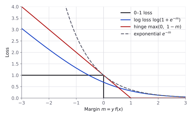
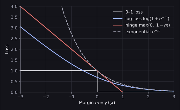
For binary score-based classification, code labels as and define the margin
A positive margin is correct, a negative margin is wrong, and a large positive margin is confidently or safely correct. In scikit-learn, decision_function returns such scores for compatible estimators.
Zero–one loss
| Field | Zero–one loss |
|---|---|
| Task and output | Classification; a predicted class or signed score |
| Formula | if , otherwise 0 |
| Target | The class decision with the smallest classification error |
| Error shape | A step: all wrong predictions cost 1 and all correct ones cost 0 |
| Robustness and symmetry | Does not distinguish slightly wrong from confidently wrong |
| Smoothness | Flat almost everywhere and discontinuous at the boundary |
| Probabilistic meaning | None directly |
| Main controls | Decision threshold |
| Use when | Describing classification error as a concept or metric |
| Be careful when | Training with gradients; it provides almost no useful direction |
Zero–one loss explains what accuracy counts, but its poor optimisation behaviour motivates the surrogate losses below.
Binary cross-entropy or log loss
For a probability and label ,
With signed labels and margin , the same loss is .
| Field | Binary cross-entropy / log loss |
|---|---|
| Task and output | Binary classification; probability or raw logit |
| Formula | Negative log-probability assigned to the observed class |
| Target | True conditional class probability |
| Error shape | Smooth; confident wrong predictions receive a very large loss |
| Robustness and symmetry | Symmetric between the two class labels, but sensitive to confidently wrong or noisy labels |
| Smoothness | Smooth and well suited to gradient training |
| Probabilistic meaning | Bernoulli negative log-likelihood |
| Main controls | Sample/class weights and any later decision threshold |
| Use when | Probabilities are needed or as a strong default binary-classification loss |
| Be careful when | Labels are noisy or raw probabilities are passed to logarithms without numerical safeguards |
Multiclass cross-entropy
If the model predicts probabilities for classes and the true class is ,
| Field | Multiclass cross-entropy |
|---|---|
| Task and output | Multiclass classification; a probability distribution over classes |
| Formula | Negative log-probability of the true class |
| Target | Conditional probability of every class |
| Error shape | Confidently assigning little probability to the true class is heavily penalised |
| Robustness and symmetry | Treats class names symmetrically unless weights are added; sensitive to incorrect labels |
| Smoothness | Smooth when applied to logits through softmax |
| Probabilistic meaning | Categorical negative log-likelihood |
| Main controls | Class/sample weights |
| Use when | Standard multiclass probability prediction |
| Be careful when | Classes have unequal costs or labels contain substantial noise |
This is the loss used by multiclass logistic regression.
Hinge loss
| Field | Hinge loss |
|---|---|
| Task and output | Binary margin-based classification; score |
| Formula | |
| Target | A separating boundary with a margin, not calibrated probabilities |
| Error shape | Linear until margin 1, then zero |
| Robustness and symmetry | Penalises wrong and boundary-adjacent samples; grows linearly for bad errors |
| Smoothness | Continuous but not differentiable at |
| Probabilistic meaning | No direct likelihood interpretation |
| Main controls | Regularisation strength and class/sample weights |
| Use when | SVM-style separation is wanted and probabilities are unnecessary |
| Be careful when | The application needs calibrated probabilities |
A correctly classified sample with still has positive hinge loss because it lies inside the desired safety margin.
Exponential loss
| Field | Exponential loss |
|---|---|
| Task and output | Binary margin-based classification; score |
| Formula | |
| Target | A class-separating score |
| Error shape | Decreases exponentially with margin and grows extremely quickly for negative margins |
| Robustness and symmetry | Very sensitive to badly misclassified or noisy samples |
| Smoothness | Smooth |
| Probabilistic meaning | Used as the optimisation view behind AdaBoost |
| Main controls | Learner weights, sample weights and boosting settings |
| Use when | Understanding or reproducing AdaBoost-style training |
| Be careful when | Outliers or incorrect labels can dominate |
For each extra unit of negative margin, exponential loss is multiplied by .
Comparing the margin losses
| Margin | −2 | −1 | 0 | 0.5 | 1 | 2 |
|---|---|---|---|---|---|---|
| Zero–one | 1 | 1 | 1 | 0 | 0 | 0 |
| Log loss | 2.127 | 1.313 | 0.693 | 0.474 | 0.313 | 0.127 |
| Hinge | 3 | 2 | 1 | 0.5 | 0 | 0 |
| Exponential | 7.389 | 2.718 | 1 | 0.607 | 0.368 | 0.135 |
The table and figure show why “classification loss” is not one behaviour. Hinge loss stops caring after margin 1, log loss continues to reward greater confidence gently, and exponential loss lets badly misclassified samples dominate.
OptionalWorked example: scores, probabilities and hinge loss
Suppose samples with identical features share one score , and a fraction has positive labels. The code finds the score that minimises log and hinge loss.
f = np.linspace(-5, 5, 100001)
for p in [0.7, 0.9]:
    log = p * np.log(1 + np.exp(-f)) + (1 - p) * np.log(1 + np.exp(f))
    hinge = p * np.maximum(0, 1 - f) + (1 - p) * np.maximum(0, 1 + f)
    f_log, f_hinge = f[np.argmin(log)], f[np.argmin(hinge)]
    p_back = 1 / (1 + np.exp(-f_log))
    print(p, round(f_log, 3), round(p_back, 3), round(f_hinge, 3))
# 0.7 0.847 0.7 1.0
# 0.9 2.197 0.9 1.0
Log loss chooses the log-odds, whose sigmoid recovers . Hinge loss chooses 1 in both cases: it records which class is more frequent, but not by how much.
from sklearn.datasets import load_breast_cancer
from sklearn.linear_model import SGDClassifier
from sklearn.model_selection import train_test_split
from sklearn.pipeline import make_pipeline
from sklearn.preprocessing import StandardScaler

X, y = load_breast_cancer(return_X_y=True)
X_train, X_test, y_train, y_test = train_test_split(
    X, y, test_size=0.2, stratify=y, random_state=0
)
for loss in ["hinge", "log_loss"]:
    clf = make_pipeline(
        StandardScaler(), SGDClassifier(loss=loss, random_state=0)
    )
    clf.fit(X_train, y_train)
    print(loss, round(clf.score(X_test, y_test), 3),
          hasattr(clf, "predict_proba"))
# hinge 0.965 False
# log_loss 0.965 True
Both reach accuracy 0.965, but only the log-loss model provides predict_proba. Likewise, XGBoost's "binary:hinge" predicts hard labels, while "binary:logistic" predicts probabilities.
OptionalProbabilistic interpretation of losses
Choosing a loss can be interpreted as choosing an assumption about how the data is generated.
Suppose a regression label equals the model prediction plus independent noise:
Training can choose the parameters that make the observed labels most likely. Maximising this likelihood is equivalent to minimising its negative logarithm.
- Gaussian noise. If has density , the negative log-likelihood is squared error divided by , plus a constant.
- Laplace noise. With density , the negative log-likelihood is absolute error divided by , plus a constant.
- Bernoulli labels. If with probability , the negative log-likelihood is binary cross-entropy.
For , a residual of 4 is times as likely as zero under Laplace noise, but only times as likely under Gaussian noise. The heavier Laplace tails make large errors less surprising, which matches the greater robustness of absolute error.
The important conclusion is not the density algebra: choosing a loss also chooses assumptions about label noise or uncertainty.
Weighted losses
Weighting is not a separate loss family. It modifies any existing loss by deciding which samples matter more:
A sample with a larger non-negative weight has more influence on the fitted parameters. The underlying loss could be squared error, cross-entropy, hinge loss or something else.
Sample weights and class weights
- A sample weight assigns importance to one particular training example.
- A class weight gives the same weight to every example of one class.
Scikit-learn commonly accepts weights through fit(X, y, sample_weight=w). For LogisticRegression, weight 2 on one sample produces the same fitted model as including that sample twice.
OptionalCheck that a sample weight acts like repetition
from sklearn.datasets import load_breast_cancer
from sklearn.linear_model import LogisticRegression
from sklearn.preprocessing import StandardScaler

X, y = load_breast_cancer(return_X_y=True)
X = StandardScaler().fit_transform(X)
X_rep = np.vstack([X, X[:1]])
y_rep = np.append(y, y[0])
w = np.ones(len(y))
w[0] = 2

opts = dict(tol=1e-10, max_iter=10_000)
a = LogisticRegression(**opts).fit(X_rep, y_rep)
b = LogisticRegression(**opts).fit(X, y, sample_weight=w)
print(np.allclose(a.coef_, b.coef_),
np.allclose(a.intercept_, b.intercept_)) # True TrueWith class_weight="balanced", scikit-learn gives class the weight
where is the number of classes and is the number of samples in class . Every class then has the same total weight, .
OptionalWorked example: class weights on imbalanced data
from sklearn.datasets import make_classification
from sklearn.metrics import precision_score, recall_score
from sklearn.model_selection import train_test_split
from sklearn.pipeline import make_pipeline
from sklearn.utils.class_weight import compute_class_weight

X, y = make_classification(
    n_samples=2000, n_features=10, n_informative=4, n_redundant=0,
    weights=[0.9], class_sep=1.5, random_state=0,
)
X_train, X_test, y_train, y_test = train_test_split(
    X, y, test_size=0.25, stratify=y, random_state=0
)

print(np.bincount(y_train))
print(compute_class_weight(
    "balanced", classes=np.array([0, 1]), y=y_train
).round(3))

for cw in [None, "balanced"]:
    clf = make_pipeline(
        StandardScaler(), LogisticRegression(class_weight=cw)
    )
    clf.fit(X_train, y_train)
    pred = clf.predict(X_test)
    print(cw, round(recall_score(y_test, pred), 3),
          round(precision_score(y_test, pred), 3))
# [1337  163]
# [0.561 4.601]
# None 0.204 0.846
# balanced 0.63 0.209
Class 1 receives about 8.2 times the weight of class 0. Recall rises from 0.204 to 0.630, while precision falls from 0.846 to 0.209. Balanced accuracy rises from 0.600 to 0.670 and ordinary accuracy falls from 0.910 to 0.702.
Weighting therefore changes the tradeoff; it does not make every metric better. Lowering the decision threshold of the unweighted model can have a similar effect.
Loss and evaluation metric
Training needs a quantity that can guide optimisation. Evaluation needs a quantity that reflects the task's goal. Sometimes one function can do both jobs; sometimes a smooth surrogate and a later decision rule are needed.
| Evaluation goal | Useful training approach |
|---|---|
| MSE or RMSE | Squared error |
| Mean absolute error | Absolute error, or Huber for a smoother robust compromise |
| A quantile or prediction interval | Pinball loss at the required level or levels |
| Log loss or probability quality | Cross-entropy / log loss |
| Accuracy or F1 | Log or hinge loss, then choose the class threshold on validation data |
| ROC AUC | Train a score-producing model, then evaluate its ranking |
| Sample- or class-weighted metric | Apply matching weights to a suitable base loss |
Accuracy, F1 and ROC AUC change in steps as predictions change, so gradient methods do not directly minimise them. Train with a surrogate, then tune any threshold on validation data as described in Model Evaluation Metrics.
The same loss ideas appear across model families:
- Decision trees use split criteria related to the prediction error in their leaves. Squared and absolute regression criteria produce means and medians; classification impurity is covered in Decision Trees.
- Gradient boosting fits new trees using derivatives of the chosen loss, as shown in XGBoost.
- Neural networks use the same principles through functions such as
nn.MSELoss,nn.L1Lossandnn.CrossEntropyLoss. The deep-learning loss module will build on this framework.
Choosing a loss
The cards provide detail; this decision flow gives a practical starting point.
Regression
├─ Need the ordinary conditional average? → squared error
├─ Need the median or stronger outlier resistance? → absolute error
├─ Want smooth small-error fitting with robust tails? → Huber
└─ Need a quantile, interval or asymmetric penalty? → pinball

Classification
├─ Need probabilities? → binary or multiclass cross-entropy
├─ Need only a separating boundary? → hinge is possible
└─ Using AdaBoost-style training? → exponential loss

Unequal sample or class importance? → weight the chosen loss
Step-based metric such as F1?        → train a surrogate, tune threshold later
The default loss is usually a sensible baseline. Change it when the target quantity, outlier behaviour, direction of error, probability requirement or metric gives a specific reason.
OptionalLibrary names for the catalogue
Library names are reference material rather than new loss concepts. Defaults and supported strings can vary by estimator.
| Conceptual loss | scikit-learn examples | XGBoost objective |
|---|---|---|
| Squared error | LinearRegression; loss="squared_error" in SGDRegressor, HistGradientBoostingRegressor, GradientBoostingRegressor |
"reg:squarederror" |
| Absolute error | QuantileRegressor(quantile=0.5); loss="absolute_error" in gradient-boosting regressors; criterion="absolute_error" in DecisionTreeRegressor |
"reg:absoluteerror" |
| Huber | HuberRegressor; loss="huber" in SGDRegressor and GradientBoostingRegressor |
"reg:pseudohubererror" with huber_slope |
| Pinball | QuantileRegressor(quantile=τ); quantile losses in gradient-boosting regressors |
"reg:quantileerror" with quantile_alpha=τ |
| Binary log loss | LogisticRegression; SGDClassifier(loss="log_loss") |
"binary:logistic" |
| Multiclass cross-entropy | Multinomial LogisticRegression |
"multi:softprob" |
| Hinge | SGDClassifier(loss="hinge"); LinearSVC(loss="hinge") |
"binary:hinge" returns hard labels |
| Exponential | GradientBoostingClassifier(loss="exponential") |
AdaBoost-style rather than the standard XGBoost objective |
LinearSVC defaults to squared hinge rather than hinge. PyTorch expresses the same core families with nn.MSELoss, nn.L1Loss, nn.HuberLoss, nn.BCEWithLogitsLoss and nn.CrossEntropyLoss.
The whole idea in one view
loss for one prediction
        ↓ average across samples
training cost
        ↓ add any parameter penalty
objective minimised by training

choosing the loss decides
├─ what quantity the model predicts
├─ how quickly penalties grow
├─ whether outliers dominate
├─ whether error direction matters
└─ what optimisation signal the model receives

weights modify an existing loss
metric evaluates the final behaviour
Once these questions are understood, a new loss is no longer an isolated formula. It is another card in the same framework.
Resources
| Source | Title | Why read it |
|---|---|---|
| scikit-learn | User Guide: Stochastic Gradient Descent | The section “Mathematical formulation” gives the formula of every loss available in SGDClassifier and SGDRegressor, including hinge, log loss and Huber. |
| scikit-learn | SGD: convex loss functions | A short script that plots the zero-one, hinge, log and other classification losses against the decision score of a sample with label 1. Its log loss uses base-2 logarithms. |
| scikit-learn | User Guide: Linear Models | The sections “Huber Regression” and “Quantile Regression” state the exact objectives of HuberRegressor and QuantileRegressor, including the scale estimate of the first and the L1 penalty of the second. |
| scikit-learn | HuberRegressor vs Ridge on dataset with strong outliers | Shows the Huber fit moving towards the ridge fit as epsilon increases. |
| Google for Developers | Linear regression: Loss | “Types of loss” and “Choosing a loss” compare squared and absolute loss and how each treats outliers. |
| XGBoost | XGBoost Parameters | “Learning Task Parameters” lists every objective string, followed by the parameters of the pseudo-Huber and quantile losses. |
Practice problems
| Solved | Source | Problem | Difficulty | Tags |
|---|---|---|---|---|
| IOAI 2025 | Radar (at-home) | Medium | segmentation, imbalanced classes | |
| IOAI 2025 | Chicken Counting | Hard | vision, regression |
Finished this module? Mark it done.
Comments
Stuck on something, spotted a mistake, or found a resource that helped you? Tell us below.
Loading comments