4Classical Machine Learning 4.5Classical Machine Learning Models
4.5.7 K-Means Clustering
An unsupervised method that partitions samples into k clusters, each represented by the mean of its samples, by minimising the sum of squared distances from samples to their cluster means.
What clustering does
The models so far have learned from labelled examples. They receive features together with a known answer , then learn how to predict that answer for a new sample.
Sometimes there is no . We may have customer records, image measurements or sensor readings without knowing which group each sample belongs to. We can still ask whether samples with similar features naturally gather into groups.
features X
    ↓
group similar samples together
    ↓
clusters
This is clustering, a form of unsupervised learning. K-means is one of the simplest and most widely used clustering methods. It represents every group by a centre and places each sample with the centre nearest to it.
K-means is not K-NN
Their names are easy to confuse, but they solve different problems.
| K-NN | K-means | |
|---|---|---|
| Type of learning | Supervised | Unsupervised |
| Training labels | Requires | Uses only |
| Meaning of | Number of neighbours | Number of clusters |
| Main purpose | Predict a label or value | Discover groups |
The basic idea
Consider six points with two features:
| Sample | First feature | Second feature |
|---|---|---|
| 1 | 1 | |
| 3 | 1 | |
| 2 | 4 | |
| 6 | 5 | |
| 8 | 5 | |
| 7 | 8 |
The first three sit around the lower-left of a graph, while the last three sit around the upper-right. If we choose , we are asking K-means to find two groups.
Its core idea is:
choose 2 centres
        ↓
assign every point to its nearest centre
        ↓
move each centre to the middle of its group
        ↓
repeat until the groups stop changing
The same process works for any chosen value of .
Centroids: the centres of the clusters
Each cluster is represented by a centroid, which is the mean of all the points assigned to that cluster.
For example, the centroid of , and is
Notice that the centroid is calculated from the samples; it does not have to be one of the actual samples.
Using the notation from earlier, the centroid of cluster is
where is the number of samples in that cluster.
What makes a clustering good?
K-means tries to keep every sample close to the centroid of its own cluster. For one sample, it measures the squared Euclidean distance
It then adds these distances across all samples. This total is called inertia, or the within-cluster sum of squares:
Smaller inertia means that the samples are packed more tightly around their centroids. K-means searches for a clustering with low inertia.
Inertia falls as more clusters are added, so it cannot choose by itself. We will return to this in Choosing the number of clusters.
For our six points, the natural groups have centroids and . Their squared distances from the first centroid are 2, 2 and 4; those from the second are also 2, 2 and 4. The final inertia is therefore
OptionalOptional mathematics: why K-means uses the mean
K-means is built around squared Euclidean distance. For a fixed group of points, the value of
is smallest when is the mean of the points. This is the same reason that a regression-tree leaf predicts the mean when it uses squared error.
The choice of distance and the choice of centre are connected. If the objective used a different idea of distance, the mean might no longer be the correct centre.
The K-means algorithm
There are ways to place samples into clusters, so trying every possible grouping quickly becomes impossible. K-means instead starts with a guess and improves it repeatedly. This procedure is called Lloyd's algorithm.
choose k starting centroids

repeat:
    assignment step:
        assign each sample to its nearest centroid

    update step:
        replace each centroid with the mean of its samples

until the assignments stop changing
The two steps have simple jobs:
- Assignment: decide which centre each sample belongs to.
- Update: move each centre to the middle of its newly assigned samples.
Then K-means assigns again using the moved centres, updates again, and continues until the clustering settles.
One iteration by hand
Start the six-point example with both centroids in the lower-left group:
The assignment step compares the squared distance from every point to both centres:
| Sample | To | To | Assigned cluster |
|---|---|---|---|
| 0 | 10 | 1 | |
| 4 | 10 | 1 | |
| 10 | 0 | 2 | |
| 41 | 17 | 2 | |
| 65 | 37 | 2 | |
| 85 | 41 | 2 |
The update step now takes the mean of each group:
The centres have moved from their original positions to the middles of their assigned groups. The next iteration repeats the same two steps using these new centres.
OptionalOptional: finish the example by hand
With the starting centroids, the first assignments have inertia
Moving the centres to and lowers it to 31.75. In the second assignment, is at squared distance 9 from the first centroid and 16.3125 from the second, so it moves to cluster 1.
The next update gives
with inertia 16. In the third iteration no sample moves, so the algorithm stops.
import numpy as np
from sklearn.cluster import KMeans

X = np.array([[1, 1], [3, 1], [2, 4],
              [6, 5], [8, 5], [7, 8]])
start = np.array([[1, 1], [2, 4]])

km = KMeans(n_clusters=2, init=start, n_init=1).fit(X)
print(km.labels_)               # [0 0 0 1 1 1]
print(km.cluster_centers_)      # [[2. 2.]
                                #  [7. 6.]]
print(km.inertia_, km.n_iter_)  # 16.0 3
Scikit-learn numbers clusters from 0 rather than 1, but the grouping is the same.
Using KMeans in practice
Scikit-learn follows the same estimator interface as its other models, with one important difference: fit receives only X because there are no target labels.
import numpy as np
from sklearn.cluster import KMeans

X = np.array([[1, 1], [3, 1], [2, 4],
              [6, 5], [8, 5], [7, 8]])

km = KMeans(n_clusters=2, n_init=10, random_state=0)
labels = km.fit_predict(X)

print(labels)               # cluster of each training sample
print(km.cluster_centers_)  # learned centroids
print(km.inertia_)          # final inertia
print(km.n_iter_)           # iterations used by the best run
The main fitted results are:
| Attribute or method | What it gives you |
|---|---|
fit_predict(X) |
Fits the model and returns a cluster for every row of X |
cluster_centers_ |
The learned centroids |
labels_ |
The cluster assigned to each training sample |
inertia_ |
The final sum of squared distances |
n_iter_ |
The number of iterations used |
predict(X_new) |
The nearest fitted cluster for each new sample |
transform(X_new) |
Each sample's distance to every centroid |
Cluster numbers are only names. Cluster 0 is not inherently better, earlier or more meaningful than cluster 1.
Why every iteration helps
Each part of the algorithm can only keep inertia the same or lower it:
- During assignment, every sample moves to its nearest available centroid.
- During updating, every centroid moves to the mean, the point that gives its cluster the smallest squared distance.
K-means therefore keeps moving downhill until the assignments stop changing.
OptionalOptional proof: why Lloyd's algorithm stops
When a sample changes cluster, it moves to a strictly closer centroid, so inertia decreases. Updating a centroid to the mean also cannot increase inertia.
There are only finitely many ways to assign samples to clusters. Because every genuine change reduces inertia, the algorithm cannot cycle through the same assignments forever. It must eventually stop.
A stable answer is not always the best answer
K-means can settle into a grouping where neither step changes anything even though a better grouping exists. This is called a local minimum.
For example, consider the four corners , , and with :
- Grouping the left pair and right pair gives inertia 1.
- Grouping the bottom pair and top pair gives inertia 16.
The second grouping is much worse, but it is locally stable: every point is still closer to its current centroid than the other one. Different starting centroids can therefore lead K-means to different final answers.
The essential lesson is:
different starting centres
        ↓
different paths through the algorithm
        ↓
possibly different final clusters
Better starting points with K-means++
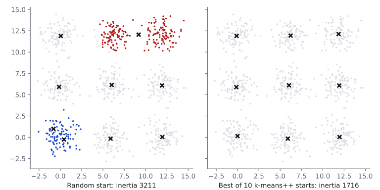
With completely random starts, several centroids may begin in one natural group while another group gets none. Scikit-learn therefore uses init="k-means++" by default.
K-means++ chooses the first centre, then gives points far from the centres already chosen a greater chance of becoming the next centre. This tends to spread the starting centroids across the dataset and usually gives Lloyd's algorithm a much better starting point.
OptionalOptional mathematics: exact K-means++ sampling
Let be the distance from to its nearest centre chosen so far. The next point is selected with probability proportional to its squared distance:
In the six-point example, suppose is the first centre. The squared distances are 0, 4, 10, 41, 65 and 85, with total 205. The chance that the second centre comes from the upper-right group is therefore
compared with if it were drawn uniformly from the other five points.
Scikit-learn uses a greedy variant. At each step it samples candidates with this weighting and keeps the candidate that lowers inertia the most.
Try several starts
Even K-means++ can occasionally start badly. A common safeguard is to run the entire algorithm several times and keep the result with the smallest inertia.
Two settings control different parts of this process:
initdecides how one run chooses its starting centroids.n_initdecides how many separate runs are tried.
With n_init="auto", scikit-learn uses 10 runs for init="random" and one run for init="k-means++".
OptionalOptional experiment: initialization and multiple starts
The following experiment clusters 900 samples from nine well-separated blobs using 100 random seeds for each setting.
from sklearn.datasets import make_blobs

grid = np.array([[i, j] for i in range(3) for j in range(3)]) * 6.0
Xb, yb = make_blobs(
    n_samples=900, centers=grid, cluster_std=1.0, random_state=0
)

def inertias(**params):
    return np.array([
        KMeans(n_clusters=9, random_state=seed, **params)
        .fit(Xb).inertia_
        for seed in range(100)
    ])

for init, n_init in [
    ("random", 1), ("k-means++", 1),
    ("random", 10), ("k-means++", 10),
]:
    J = inertias(init=init, n_init=n_init)
    print(init, n_init, np.median(J), J.max(), (J < 1716).sum())
init |
n_init |
Median inertia | Largest inertia | Seeds reaching 1715.9 |
|---|---|---|---|---|
"random" |
1 | 3317.7 | 5177.7 | 26 of 100 |
"k-means++" |
1 | 1715.9 | 3388.1 | 89 of 100 |
"random" |
10 | 1715.9 | 3220.1 | 96 of 100 |
"k-means++" |
10 | 1715.9 | 1715.9 | 100 of 100 |
The lowest inertia corresponds to one centroid per blob. One random start reaches it for only 26 seeds, while ten K-means++ starts reach it for all 100 in this experiment. More starts cost more computation, but reduce the chance of keeping a poor local minimum.
Choosing the number of clusters
K-means requires us to choose n_clusters before training. This hyperparameter can be difficult to choose precisely because clustering has no labels to validate against.
Why inertia alone cannot choose
Adding more centroids can only make samples closer to a centre, so the smallest possible inertia always falls as grows. At the extreme, gives every sample its own centroid and inertia becomes 0.
The value of with the smallest inertia is therefore not automatically the most useful choice.
The elbow method
The elbow method fits K-means for several values of and plots against inertia.
first few extra clusters
→ large drop in inertia

later extra clusters
→ only small improvements
The bend between these two patterns is the elbow and suggests a possible value of . It is a visual heuristic, not an exact rule; some datasets have no clear elbow.
Silhouette score
The silhouette score asks whether a sample is closer to its own cluster than to the neighbouring clusters.
For sample :
- is its average distance to the other points in its own cluster.
- is its smallest average distance to the points in another cluster.
Its silhouette value is
| Silhouette value | Interpretation |
|---|---|
| Near 1 | Fits its own cluster well and is far from other clusters |
| Near 0 | Lies near the boundary between clusters |
| Below 0 | May fit another cluster better |
The overall silhouette score is the mean across all samples. Higher values generally mean cleaner separation.
OptionalOptional: calculate one silhouette value by hand
For in the six-point example, its distances to and are both , so .
Its mean distance to the other cluster is
Therefore,
Scikit-learn provides both per-sample values and their average:
from sklearn.metrics import silhouette_samples, silhouette_score

print(silhouette_samples(X, km.labels_).round(4))
# [0.6731 0.6022 0.4288 0.5013 0.6232 0.5995]
print(round(silhouette_score(X, km.labels_), 4))  # 0.5713
Silhouette uses ordinary distances, not squared distances.
Use both signals
It is often useful to inspect both inertia and silhouette score:
from sklearn.datasets import make_blobs
from sklearn.metrics import silhouette_score

Xc, yc = make_blobs(n_samples=600, centers=4, random_state=42)

for k in range(1, 8):
    fitted = KMeans(n_clusters=k, n_init=10, random_state=0).fit(Xc)
    sil = silhouette_score(Xc, fitted.labels_) if k > 1 else float("nan")
print(k, round(fitted.inertia_, 1), round(sil, 3))| 1 | 2 | 3 | 4 | 5 | 6 | 7 | |
|---|---|---|---|---|---|---|---|
| Inertia | 39698.3 | 18637.9 | 4178.9 | 1160.3 | 1045.8 | 938.4 | 844.2 |
| Silhouette | — | 0.591 | 0.757 | 0.788 | 0.691 | 0.559 | 0.427 |
Here the inertia has an elbow at , and the silhouette score is also highest there. That is useful evidence for four clusters, but neither measure guarantees that those clusters have the real-world meaning we want.
A cluster is not automatically a class
K-means sees only distances between feature values. It does not know what a flower species, customer type or authentic painting means.
cluster = a geometric pattern in the chosen features
class   = a meaningful target defined by the problem
Those ideas may line up, but they do not have to. The Iris dataset has three named species, for example, yet its silhouette score prefers because two of the species overlap geometrically.
| Silhouette score | ARI with the three species | |
|---|---|---|
| 2 | 0.681 | 0.540 |
| 3 | 0.553 | 0.730 |
| 4 | 0.498 | 0.650 |
| 5 | 0.489 | 0.608 |
The two-cluster solution separates the 50 setosa flowers and 3 versicolor flowers from the overlapping versicolor and virginica flowers. The geometry is reasonable, even though it does not reproduce all three species.
OptionalOptional: comparing clusters with known labels
If labels happen to be available, the adjusted Rand index (ARI) compares the grouping formed by the clusters with the grouping formed by the labels.
- 1 means that the two groupings match perfectly.
- A value around 0 means roughly chance-level agreement.
- Cluster numbers themselves do not matter:
[0, 0, 1, 1]and[1, 1, 0, 0]describe the same grouping.
The ordinary Rand index checks pairs of samples: did both groupings put the pair together, or did both keep it apart? ARI adjusts this score for agreements that could happen by chance.
from sklearn.datasets import load_iris
from sklearn.metrics import adjusted_rand_score, silhouette_score

iris = load_iris()
for k in range(2, 6):
    labels = KMeans(
        n_clusters=k, n_init=10, random_state=0
    ).fit_predict(iris.data)
    print(
        k,
        round(silhouette_score(iris.data, labels), 3),
        round(adjusted_rand_score(iris.target, labels), 3),
    )

print(adjusted_rand_score([0, 0, 1, 1], [1, 1, 0, 0])) # 1.0Feature scaling changes what “close” means
K-means uses Euclidean distance. A feature with a large numerical range can therefore dominate the distance and decide the clusters almost by itself.
Imagine two features:
height: 1.5 to 1.9 metres
income: 30,000 to 70,000
A difference of several thousand in income overwhelms a difference of a few tenths in height. StandardScaler changes each feature to
putting their numerical scales on a more comparable footing.
This is the same issue seen with K-NN: distance decides the neighbours in K-NN and the nearest centroid in K-means.
OptionalExample: clustering before and after scaling
The six people below form two groups by height. Their incomes are unrelated to those groups.
| Person | Height (m) | Income |
|---|---|---|
| 0 | 1.58 | 52,000 |
| 1 | 1.61 | 31,000 |
| 2 | 1.63 | 66,000 |
| 3 | 1.79 | 38,000 |
| 4 | 1.81 | 59,000 |
| 5 | 1.84 | 45,000 |
import pandas as pd
from sklearn.pipeline import make_pipeline
from sklearn.preprocessing import StandardScaler

people = pd.DataFrame({
    "height_m": [1.58, 1.61, 1.63, 1.79, 1.81, 1.84],
    "income": [52_000, 31_000, 66_000, 38_000, 59_000, 45_000],
})

kmeans = KMeans(n_clusters=2, n_init=10, random_state=0)
raw = kmeans.fit_predict(people)
scaled = make_pipeline(StandardScaler(), kmeans).fit_predict(people)
print(raw, scaled) # [1 0 1 0 1 0] [1 1 1 0 0 0]| Person | Cluster without scaling | Cluster after scaling |
|---|---|---|
| 0 | 1 | 1 |
| 1 | 0 | 1 |
| 2 | 1 | 1 |
| 3 | 0 | 0 |
| 4 | 1 | 0 |
| 5 | 0 | 0 |
Without scaling, income controls the groups. After scaling, the result matches the two height groups. In a similar generated dataset with 200 people, the ARI with the height groups is 0.007 without scaling and 1.0 after scaling.
Standardisation is often a sensible starting point when units or ranges differ greatly, but it is still a modelling choice—not an automatic rule. Scaling decides the relative importance of the features. On Iris, where all four features are lengths measured in centimetres, standardising lowers the ARI for three clusters from 0.73 to 0.62.
What kinds of clusters does K-means expect?
K-means works best when the groups are roughly:
- compact and blob-like;
- similarly spread;
- clearly separated; and
- meaningful under Euclidean distance.
Every sample joins the closest centroid, so each cluster becomes the region closest to one centre. These regions are convex. This fits round blobs well, but it cannot naturally make one curved group wrap around another.
K-means can struggle with:
- crescent-shaped clusters such as two moons;
- rings or other interleaving shapes;
- long, tilted clusters;
- groups with very different spreads or sizes; and
- outliers, which can pull a mean far from most of its cluster.
Most importantly, K-means can minimise its own objective successfully and still find the “wrong” groups. In that case the optimisation did not fail—the assumptions behind the objective did not match the data.
OptionalOptional experiment: curved and elongated clusters
from sklearn.cluster import DBSCAN
from sklearn.datasets import make_blobs, make_moons
from sklearn.metrics import adjusted_rand_score
from sklearn.mixture import GaussianMixture

Xm, ym = make_moons(n_samples=400, noise=0.05, random_state=0)
moons = KMeans(n_clusters=2, n_init=10, random_state=0).fit(Xm)
print(round(adjusted_rand_score(ym, moons.labels_), 3))  # 0.274

Xa, ya = make_blobs(n_samples=600, centers=3, random_state=170)
Xa = Xa @ np.array([[0.6, -0.6], [-0.4, 0.8]])
aniso = KMeans(n_clusters=3, n_init=10, random_state=0).fit(Xa)

true_J = sum(
    ((Xa[ya == j] - Xa[ya == j].mean(axis=0)) ** 2).sum()
    for j in range(3)
)
print(round(adjusted_rand_score(ya, aniso.labels_), 3))  # 0.58
print(round(aniso.inertia_, 1), round(true_J, 1))        # 690.8 876.9

db = DBSCAN(eps=0.2).fit_predict(Xm)
gm = GaussianMixture(n_components=3, random_state=0).fit_predict(Xa)
print(
    round(adjusted_rand_score(ym, db), 3),
    round(adjusted_rand_score(ya, gm), 3),
)  # 1.0 1.0
K-means scores only 0.274 ARI on the two moons and 0.58 on the stretched blobs. On the blobs, its clustering even has lower inertia than the true groups—690.8 instead of 876.9. This clearly shows that the K-means objective, rather than the way it was optimised, is unsuitable for those shapes.
OptionalOptional: other clustering methods
Other methods make different assumptions:
- DBSCAN builds clusters from points connected through dense neighbourhoods. It can follow curved shapes and does not require , although its own settings still matter. It separates the moons above with
eps=0.2; with its defaulteps=0.5, it puts all 400 points in one cluster. - Gaussian mixtures allow elliptical clusters. Each component has a covariance matrix and recovers the stretched blobs above.
- Spectral clustering can capture more complicated geometric structure, including some curved or interleaved groups.
These methods are mentioned here as contrasts. Each deserves its own careful treatment before use.
Useful KMeans settings
| Setting | Default | Meaning |
|---|---|---|
n_clusters |
8 |
How many clusters to form |
init |
"k-means++" |
How one run chooses its starting centres |
n_init |
"auto" |
How many starting configurations to try |
max_iter |
300 |
Maximum updates in each run |
random_state |
None |
Reproducibility of the starting centres |
OptionalOptional: more KMeans settings and methods
| Setting or method | Meaning |
|---|---|
tol=1e-4 |
Stops when the total squared movement of the centroids is at most tol times the mean feature variance |
algorithm="lloyd" |
Uses the standard algorithm explained above |
algorithm="elkan" |
Uses the triangle inequality to skip some distance calculations, at a higher memory cost |
score(X) |
Returns the negative inertia, so a larger score means smaller inertia |
Here is a fuller look at the fitted outputs on Iris:
from sklearn.datasets import load_iris

iris = load_iris()
km_iris = KMeans(n_clusters=3, random_state=0).fit(iris.data)

print(km_iris.cluster_centers_.round(2))
# [[5.88 2.74 4.39 1.43]
#  [5.01 3.43 1.46 0.25]
#  [6.85 3.08 5.72 2.05]]

print(km_iris.labels_[:5], np.bincount(km_iris.labels_))
# [1 1 1 1 1] [61 50 39]

print(round(km_iris.inertia_, 2), km_iris.n_iter_)  # 78.86 7

new = np.array([[5.0, 3.4, 1.5, 0.2], [6.5, 3.0, 5.5, 2.0]])
print(km_iris.predict(new))             # [1 2]
print(km_iris.transform(new).round(2))
# [[3.33 0.07 4.97]
#  [1.42 4.67 0.42]]

print(np.isclose(km_iris.score(iris.data), -km_iris.inertia_)) # TrueOptionalOptional: MiniBatchKMeans for large datasets
Normal K-means repeatedly uses every sample. MiniBatchKMeans updates its centroids from small random batches instead.
Its default batch_size is 1024, and partial_fit can process data in chunks. The scikit-learn User Guide says that it usually converges faster than KMeans, with a small possible loss in clustering quality. The real speed-up depends on the dataset, so measure it on the task at hand.
OptionalOptional: K-means from scratch in NumPy
def lloyd(X, centroids, max_iter=300):
    centroids = centroids.astype(float)
    labels = None

    for _ in range(max_iter):
        # Squared distance from every sample to every centroid: (n, k)
        d2 = ((X[:, None, :] - centroids[None, :, :]) ** 2).sum(axis=2)
        new_labels = d2.argmin(axis=1)

        if labels is not None and (new_labels == labels).all():
            break

        labels = new_labels
        for j in range(len(centroids)):
            if (labels == j).any():
                centroids[j] = X[labels == j].mean(axis=0)

    inertia = ((X - centroids[labels]) ** 2).sum()
    return centroids, labels, inertia
The expression X[:, None, :] - centroids[None, :, :] uses NumPy broadcasting to compare every sample with every centroid at once. If a cluster becomes empty, this version keeps its old centroid; scikit-learn relocates it.
from sklearn.datasets import load_iris

iris = load_iris()
start3 = iris.data[[0, 50, 100]]

c, lab, J = lloyd(iris.data, start3)
sk = KMeans(
    n_clusters=3, init=start3, n_init=1, tol=0
).fit(iris.data)

print(np.allclose(c, sk.cluster_centers_), (lab == sk.labels_).all())
# True True
print(round(J, 4), round(sk.inertia_, 4))  # 78.8514 78.8514
From the same start, it matches scikit-learn when tol=0 disables early stopping based on centroid movement.
Using clusters as features
After fitting centroids, transform can describe one sample using new values:
distance to centroid 1
distance to centroid 2
...
distance to centroid k
These distances contain non-linear information about where the sample lies. Another model can use them as features.
OptionalExample: centroid distances with logistic regression
The noisy half-moons have a curved boundary that a plain logistic regression model cannot follow. Distances to several centroids give the linear classifier a more useful representation.
from sklearn.datasets import make_moons
from sklearn.linear_model import LogisticRegression
from sklearn.model_selection import train_test_split
from sklearn.pipeline import make_pipeline
from sklearn.preprocessing import StandardScaler

Xn, yn = make_moons(n_samples=1000, noise=0.2, random_state=0)
Xn_tr, Xn_te, yn_tr, yn_te = train_test_split(
    Xn, yn, test_size=0.3, stratify=yn, random_state=0
)

linear = LogisticRegression().fit(Xn_tr, yn_tr)
print(round(linear.score(Xn_te, yn_te), 3))  # 0.87

with_distances = make_pipeline(
    KMeans(n_clusters=20, random_state=0),
    StandardScaler(),
    LogisticRegression(),
)
with_distances.fit(Xn_tr, yn_tr)
print(round(with_distances.score(Xn_te, yn_te), 3))  # 0.97
The Pipeline fits the centroids using training data only. Accuracy rises from 0.87 on the two raw features to 0.97 on the 20 distance features.
In Lost in Hyperspace from IOAI 2024, the final model was fixed to linear regression. The rules banned supervised feature extractors but allowed unsupervised learning, making this kind of feature construction relevant.
Using many unlabelled samples with a few labels
Suppose we have many unlabelled samples but only a few labelled ones. One simple semi-supervised idea is:
cluster all samples
        ↓
inspect the known labels inside each cluster
        ↓
give the cluster its majority known label
        ↓
pass that label to the unlabelled samples
This works only when the clusters line up with the classes. The earlier warning—cluster class—still applies.
OptionalOptional experiment: only three labelled Wine samples
The following experiment draws one labelled training sample from each Wine cultivar and repeats the draw 20 times.
from collections import Counter
from sklearn.datasets import load_wine
from sklearn.linear_model import LogisticRegression
from sklearn.model_selection import train_test_split
from sklearn.pipeline import make_pipeline
from sklearn.preprocessing import StandardScaler

wine = load_wine()
W_tr, W_te, w_tr, w_te = train_test_split(
    wine.data,
    wine.target,
    test_size=0.3,
    stratify=wine.target,
    random_state=0,
)

clusterer = make_pipeline(
    StandardScaler(),
    KMeans(n_clusters=3, n_init=10, random_state=0),
)
clusters = clusterer.fit_predict(W_tr)
test_clusters = clusterer.predict(W_te)

sup_acc, ctl_acc = [], []
for seed in range(20):
    rng = np.random.default_rng(seed)
    known = [rng.choice(np.flatnonzero(w_tr == c)) for c in range(3)]

    supervised = make_pipeline(StandardScaler(), LogisticRegression())
    supervised.fit(W_tr[known], w_tr[known])
    sup_acc.append(supervised.score(W_te, w_te))

    votes = [
        Counter(w_tr[i] for i in known if clusters[i] == c)
        for c in range(3)
    ]
    if all(votes):
        mapping = np.array([v.most_common(1)[0][0] for v in votes])
        ctl_acc.append((mapping[test_clusters] == w_te).mean())

print(round(np.mean(sup_acc), 3), round(min(sup_acc), 3),
      round(max(sup_acc), 3))
# 0.722 0.315 0.926
print(len(ctl_acc), round(np.mean(ctl_acc), 3))
# 18 0.944
Logistic regression trained on only three rows reaches a mean test accuracy of 0.722, ranging from 0.315 to 0.926. In the 18 draws where every cluster receives a known label, the cluster-based method averages 0.944.
K-means in olympiad tasks
K-means can help you:
- explore structure in unlabelled data;
- create distance-to-centroid features;
- use many unlabelled samples alongside a few labelled ones; and
- find prototypes or representative groups.
But spotting a possible clustering problem is only half the job. You must also ask whether K-means' distance and shape assumptions suit the data.
When should I try K-means?
K-means is a useful first attempt when:
- the data has no labels;
- you suspect compact natural groups;
- Euclidean distance is meaningful for the features;
- you want a quick exploratory clustering; or
- distances to representative centres could be useful features.
Be cautious when:
- the groups are curved, interleaved or highly elongated;
- their sizes or spreads differ greatly;
- outliers can pull the means;
- feature scales are arbitrary;
- there is no defensible choice of ; or
- the geometric groups may not match the concept you care about.
The whole idea in one view
problem
features X, but no labels y
        ↓
choose k initial centroids
        ↓
assign each sample to its nearest centroid
        ↓
move every centroid to its cluster mean
        ↓
repeat until the assignments settle
        ↓
keep the best result across several starts

objective: minimise squared distance to assigned centroids

choose k: inspect the elbow and silhouette score
remember: feature scales matter, cluster shape matters,
          and a cluster is not automatically a class
Exercises
Resources
| Source | Title | Why read it |
|---|---|---|
| scikit-learn | User Guide: Clustering | Read “K-means” and “Mini Batch K-Means” for the algorithm and its assumptions, and “Rand index” and “Silhouette Coefficient” under “Clustering performance evaluation”. |
| scikit-learn | KMeans | Every parameter with its default, including init and n_init, and the fitted attributes cluster_centers_, labels_, inertia_ and n_iter_. |
| scikit-learn | Demonstration of k-means assumptions | K-means on anisotropic blobs, blobs of unequal variance and unevenly sized blobs, with remedies under “Possible solutions”. |
| scikit-learn | Selecting the number of clusters with silhouette analysis on KMeans clustering | Silhouette plots for 2 to 6 clusters on synthetic blobs, and how to read them. |
| James et al. | An Introduction to Statistical Learning with Python, section 12.4 | Free book. Section 12.4.1, “K-Means Clustering”, shows that the algorithm reaches a local optimum and compares six random starts; section 12.4.3, “Practical Issues in Clustering”, discusses standardisation and the robustness of clusters. |
| Stanford CS229 | Lecture notes: The k-means clustering algorithm | Three pages showing that k-means is coordinate descent on the distortion function J, which therefore decreases monotonically but can stop at a local optimum. |
| Arthur and Vassilvitskii | k-means++: The Advantages of Careful Seeding | The paper that introduced k-means++. Section 2.2 defines the D² weighting, and Theorem 3.1 bounds the expected inertia by 8(ln k + 2) times the optimum. |
| Google for Developers | Clustering course: Advantages and disadvantages of k-means | “Disadvantages of k-means” covers the manual choice of k, the dependence on initial values, outliers and high-dimensional data. |
| StatQuest | StatQuest: K-means clustering | Runs the algorithm step by step on a small example and shows how to choose k with an elbow plot. |
Practice problems
| Solved | Source | Problem | Difficulty | Tags |
|---|---|---|---|---|
| IOAI 2025 | Antique Painting Authentication | Medium | tabular, semi-supervised, clustering |
Finished this module? Mark it done.
Comments
Stuck on something, spotted a mistake, or found a resource that helped you? Tell us below.
Loading comments