5Deep Learning 5.2Deep Learning Fundamentals
5.2.5 Activation Functions
The small non-linear functions between the layers of a network: what the common ones look like, how their gradients behave, and which one to use where.
Why do we need activation functions?
In Tensors, Matrices, and Related Mathematical Functions, we saw that a layer of a network is mostly a matrix multiplication plus a bias: . That is a linear operation. If we stack two such layers, we get , which is just another linear function of . However many layers we stack, the whole network could still only draw straight lines and flat planes. Multi-Layer Perceptrons shows this collapse happening in code.
An activation function fixes this. It is a small non-linear function applied to every value a layer produces, before the next layer sees it:
With a non-linear between the layers, stacking layers really does add power: the network can bend its decision boundaries and fit curved relationships. This page walks through the activation functions you will actually meet, how their gradients behave (which matters for training), and which one to pick in each part of a network.
You do not need to memorise every formula here. What you should take away is the shape of each function, what goes wrong with the older ones, and the simple rule for choosing.
What you need to know
By the end of this module, you should be comfortable with these ideas:
| Idea | In one line |
|---|---|
| Activation function | A non-linear function applied to each value after a layer, so stacked layers can learn curved patterns. |
| Sigmoid | Squashes any number into (0, 1); smooth, but its gradient is at most 0.25. |
| Tanh | Squashes into (−1, 1) and is centred on zero; its gradient is at most 1. |
| ReLU | Keeps positive values and turns negatives into 0; cheap, with gradient 1 for positive inputs. The usual default. |
| Leaky ReLU | Like ReLU, but negatives are multiplied by a small slope instead of being set to 0. |
| GELU | A smooth version of ReLU, used in transformer models. |
| Vanishing gradients | Gradients that shrink layer after layer until the early layers barely learn. |
| Dead ReLU | A ReLU unit whose input is always negative, so it outputs 0 and never updates. |
| Output layer | Its activation depends on the task, and in PyTorch it is usually left to the loss function. |
That is enough to read and design the networks in this guide.
Learn it properly
This page gives you a guided tour with small experiments. A proper reading adds the details and practice that make the ideas stick, so pair the two.
Pick one main course
The topic is small, so one good chapter is enough. Read it, run its code, and then come back here for the experiments.
Our pick: Dive into Deep Learning, section 5.1
Read the Activation Functions part of section 5.1 in Dive into Deep Learning. It gives the formula for ReLU, sigmoid and tanh, plots each function and its derivative with PyTorch, and is written for exactly this stage. The rest of section 5.1, on why hidden layers help, pairs well with Multi-Layer Perceptrons.
The exercises at the end of the section are worth trying, but the ones that ask for proofs are optional at this level.
If you prefer something else
- Course notes: Stanford CS231n's Commonly used activation functions covers sigmoid, tanh, ReLU and Leaky ReLU, with blunt practical advice on which to use.
- A gentle start: Google's Machine Learning Crash Course page on activation functions is visual and short.
- A video: StatQuest's ReLU In Action shows, step by step, how ReLU units bend a straight line into a curve.
- More depth on vanishing gradients: section 5.4 of Dive into Deep Learning, Vanishing Gradients. This goes further than you need for now.
A quick tour
The rest of this page shows each activation function in a line or two of PyTorch, and then two small experiments that explain why the modern choices won. Run the snippets yourself; they are short.
Where the activation goes
Let us start with one layer and one activation. The layer turns 3 input numbers into 4 values, and the activation is applied to each of those 4 values separately:
import torch
from torch import nn

torch.manual_seed(0)
layer = nn.Linear(3, 4)
x = torch.tensor([1.0, -2.0, 0.5])

z = layer(x)            # the linear part: Wx + b
a = torch.relu(z)       # the activation, value by value
print(z)
print(a)tensor([-1.4129, -0.2851, -1.1906, 0.4664], grad_fn=<ViewBackward0>)
tensor([0.0000, 0.0000, 0.0000, 0.4664], grad_fn=<ReluBackward0>)ReLU kept the one positive value and replaced the three negative ones with 0. The grad_fn part only tells us that PyTorch is tracking these values for backpropagation; you can ignore it for now.
In a whole network, we put an activation after every hidden layer. This is the pattern you will see in almost every small PyTorch model:
model = nn.Sequential(
    nn.Linear(3, 16),
    nn.ReLU(),          # activation after the first layer
    nn.Linear(16, 16),
    nn.ReLU(),          # activation after the second layer
    nn.Linear(16, 1),   # no activation after the last layer
)
Notice that the last layer has no activation. We will see why in Which activation where.
The five functions
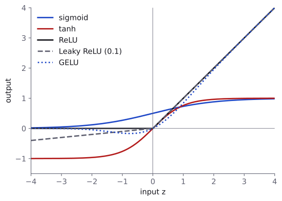
Now we can meet the functions themselves. We will feed the same five inputs to each one:
z = torch.tensor([-2.0, -0.5, 0.0, 0.5, 2.0])Sigmoid squashes any number into the range (0, 1):
torch.sigmoid(z)tensor([0.1192, 0.3775, 0.5000, 0.6225, 0.8808])You met it already in logistic regression, where it turns a score into a probability. That is still its main job today.
Tanh (the hyperbolic tangent) has the same S-shape, but squashes into (−1, 1) and is centred on 0:
torch.tanh(z)tensor([-0.9640, -0.4621, 0.0000, 0.4621, 0.9640])ReLU (rectified linear unit) keeps positive values and sets negative ones to zero:
torch.relu(z)tensor([0.0000, 0.0000, 0.0000, 0.5000, 2.0000])It is almost free to compute, which matters when a network has millions of units.
Leaky ReLU multiplies negative values by a small slope instead of setting them to 0. PyTorch's default slope is 0.01:
import torch.nn.functional as F

F.leaky_relu(z, negative_slope=0.01)tensor([-0.0200, -0.0050, 0.0000, 0.5000, 2.0000])GELU (Gaussian error linear unit) is a smooth version of ReLU. It multiplies by the probability that a standard normal variable is below , written :
F.gelu(z)tensor([-0.0455, -0.1543, 0.0000, 0.3457, 1.9545])For large positive inputs it behaves like ReLU, and for large negative ones it goes to 0, but the corner at 0 is rounded off. Transformer models, such as BERT and the GPT family, use it. You do not need the exact formula of at this level.
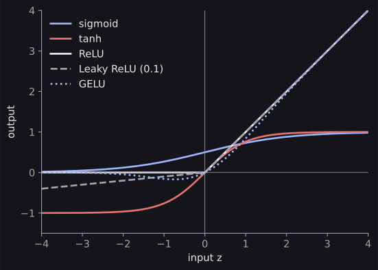
Here are all five together:
Their gradients
Training works by following gradients backwards through every layer (Backpropagation explains how). Each time the gradient passes back through an activation, it gets multiplied by that activation's derivative. So the derivative decides whether a useful signal survives the trip:
| Function | Output range | Derivative | Largest derivative |
|---|---|---|---|
| Sigmoid | (0, 1) | 0.25, at | |
| Tanh | (−1, 1) | 1, at | |
| ReLU | [0, ∞) | 1 if , else 0 | 1 |
| Leaky ReLU | (−∞, ∞) | 1 if , else | 1 |
| GELU | about [−0.17, ∞) | smooth, close to ReLU's | about 1.13 |
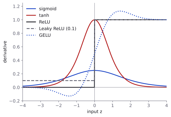
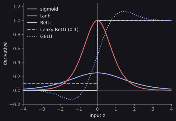
Two facts in this picture explain almost everything about choosing activations. Sigmoid's derivative is small everywhere, and sigmoid and tanh both go flat () for large inputs. ReLU's derivative, on the other hand, is exactly 1 whenever the unit is active. The next two experiments show what that means in practice.
OptionalWhere the 0.25 comes from
Write . By the chain rule,
The product of two numbers that add up to 1 is largest when both are , which happens at . So the largest possible value is .
Vanishing gradients
Let us see what a small derivative does over many layers. We pass one number through ten sigmoids in a row, then ask PyTorch how much the final output changes when the starting number changes:
start = torch.tensor(0.5, requires_grad=True)
value = start
for layer in range(10):
    value = torch.sigmoid(value)

value.backward()   # work out the gradient
print(start.grad)tensor(3.4831e-07)The gradient is about 0.00000035. Each sigmoid multiplied it by at most 0.25, and is already less than one in a million. Now the same with ReLU:
start = torch.tensor(0.5, requires_grad=True)
value = start
for layer in range(10):
    value = torch.relu(value)

value.backward()
print(start.grad)tensor(1.)With ReLU the gradient arrives untouched. In a real network the weights also scale the gradient, but the effect of the activation is the same: with sigmoid in every hidden layer, the early layers of a deep network receive almost no signal and barely learn. This is the vanishing gradient problem, and it is the main reason ReLU replaced sigmoid and tanh in hidden layers. (Good weight initialisation also matters here; it is a later, Silver-level topic.)
Dead ReLUs
ReLU has its own weakness. If a unit's input is negative for every example, it always outputs 0, its derivative is always 0, and its weights never change again. The unit is "dead". Let us build one on purpose, with a large negative bias:
weight = torch.tensor(1.0, requires_grad=True)
bias = torch.tensor(-5.0, requires_grad=True)
inputs = torch.tensor([-1.0, 0.0, 1.0, 2.0])

outputs = torch.relu(inputs * weight + bias)
outputs.sum().backward()
print(outputs)
print(weight.grad, bias.grad)tensor([0., 0., 0., 0.], grad_fn=<ReluBackward0>)
tensor(0.) tensor(0.)Every output is 0 and both gradients are 0, so gradient descent has nothing to work with. Leaky ReLU keeps a small slope for negative inputs, so the same unit still gets a gradient and can recover:
weight = torch.tensor(1.0, requires_grad=True)
bias = torch.tensor(-5.0, requires_grad=True)

outputs = F.leaky_relu(inputs * weight + bias, negative_slope=0.01)
outputs.sum().backward()
print(weight.grad, bias.grad)tensor(0.0200) tensor(0.0400)In practice, a few dead units are normal and harmless. It becomes a problem when many die at once, usually because the learning rate is too high. That is when Leaky ReLU or GELU are worth trying.
Which activation where
Now we can put it together. A network has two kinds of layers, and they follow different rules.
Hidden layers (every layer except the last) need a non-linearity so the network can learn curved patterns:
- Use ReLU by default. It is fast, and its gradient does not shrink.
- Try GELU or Leaky ReLU if training is unstable or many units seem to die. GELU is also the standard choice inside transformers.
- Avoid sigmoid and tanh in the hidden layers of ordinary networks, because of vanishing gradients. You will still see them inside some specialised layers, such as the gates of recurrent networks; those come much later.
The output layer is different. Its job is to produce the kind of answer the task needs, and in PyTorch that job is shared with the loss function:
| Task | What the last layer outputs | Activation on the last layer |
|---|---|---|
| Regression (predict a number) | One number per target, any size | None |
| Binary classification | One raw score per example | None in the model; the loss applies sigmoid internally |
| Multi-label (several yes/no labels) | One raw score per label | None in the model; the loss applies sigmoid internally |
| Multiclass (one of classes) | raw scores per example | None in the model; the loss applies softmax internally |
These raw scores are called logits. Leaving the output activation to the loss is not laziness: combining the two in one function is more numerically stable, as Loss Functions shows. When you want actual probabilities after training, apply torch.sigmoid or torch.softmax yourself.
Softmax deserves a mention here because it is the multiclass version of sigmoid: it turns scores into probabilities that add up to 1,
It is not used between layers. We look at it as a function in Tensors, Matrices, and Related Mathematical Functions, and at how the loss uses it in Loss Functions.
Activations in PyTorch
PyTorch gives you each activation in two forms, and they compute exactly the same thing:
- as a module such as
nn.ReLU(), which you put insidenn.Sequentialor store as an attribute of your model; - as a function such as
torch.relu(z)orF.relu(z)(withimport torch.nn.functional as F), which you call inside your model'sforwardmethod.
relu_module = nn.ReLU()
values = torch.tensor([-1.0, 3.0])

print(relu_module(values))
print(torch.relu(values))tensor([0., 3.])
tensor([0., 3.])Use whichever reads better in your code. The module names are the ones you would guess: nn.Sigmoid, nn.Tanh, nn.ReLU, nn.LeakyReLU, nn.GELU. The torch.nn documentation lists the rest; most of them are variations you do not need yet.
Common mistakes
| Mistake | What happens | Fix |
|---|---|---|
Writing nn.ReLU without brackets inside nn.Sequential |
TypeError: torch.nn.modules.activation.ReLU is not a Module subclass |
Write nn.ReLU(): the model needs an object, not the class. |
No activation between two nn.Linear layers |
No error, but the two layers act as one linear layer | Put an activation after every hidden layer. |
| ReLU or sigmoid after the last layer of a regression model | No error, but ReLU can never predict a negative number and sigmoid never goes above 1 | Leave the last layer of a regression model without an activation. |
Softmax or sigmoid at the end of a classifier, then nn.CrossEntropyLoss or nn.BCEWithLogitsLoss |
No error, but the function is applied twice and training becomes slower and less accurate | Output raw logits and let the loss apply it; see Loss Functions. |
| Sigmoid in every hidden layer of a deep network | Training stalls, because the early layers barely receive a gradient | Use ReLU or GELU in hidden layers. |
The last three give no error message at all, which is why they are worth remembering: the code runs, the model just learns badly.
How to practise
- Work through the Dive into Deep Learning section with its code open, and plot each function and its derivative yourself, as we did above.
- Change the experiments on this page. How small does the gradient get after 20 sigmoids? What happens to the dead ReLU if you change the bias to −0.5?
- Once you reach A Simple MLP in PyTorch, train the same network twice, once with
nn.Sigmoid()and once withnn.ReLU()in the hidden layers, and compare how fast the training loss falls.
Check yourself
What comes next
- Loss Functions: how the network's raw scores are turned into a single number that training can reduce, and why the output activation lives inside the loss.
Resources
| Source | Title | Why read it |
|---|---|---|
| Dive into Deep Learning | 5.1 Multilayer Perceptrons: Activation Functions | Our recommended main reading. Short, with the maths, plots of each function and its derivative, and PyTorch code. |
| Stanford CS231n | Neural Networks Part 1: Commonly used activation functions | Classic course notes on sigmoid, tanh, ReLU and Leaky ReLU, with practical advice. |
| Machine Learning Crash Course: Activation functions | A gentle, visual introduction. | |
| StatQuest | Neural Networks Pt. 3: ReLU In Action!!! | A short video showing how ReLU lets a network bend a straight line. |
| Dive into Deep Learning | 5.4 Numerical Stability and Initialization: Vanishing Gradients | Why sigmoid makes deep networks hard to train, in more depth. |
| PyTorch | Non-linear activations in torch.nn | The full list of activation modules, such as nn.ReLU and nn.GELU. |
Finished this module? Mark it done.
Comments
Stuck on something, spotted a mistake, or found a resource that helped you? Tell us below.
Loading comments