4Classical Machine Learning 4.5Classical Machine Learning Models
4.5.2 Logistic Regression
Turn a weighted score into class probabilities, make predictions with a threshold, and train the model with log loss.
What logistic regression does
Linear regression predicts a number. Logistic regression predicts the probability that an example belongs to a class.
For example, it can estimate the probability that:
- an email is spam;
- a tumour is malignant; or
- a sentence was generated by an AI model.
The connection with linear regression is direct:
linear regression:    features → weighted sum → predicted number
logistic regression:  features → weighted sum → sigmoid → probability
Both models begin with the same weighted score:
The score can be any real number. A probability, however, must stay between 0 and 1. Logistic regression passes the score through the sigmoid function to keep it inside that range.
Despite its name, logistic regression is a classification model. It is fast, its weights can be inspected, and it is a strong baseline for tabular data and for features created by other models.
Why not use linear regression for classes?
We could encode two classes as 0 and 1, fit linear regression, and treat values above 0.5 as class 1. The problem is that a straight line does not stay between 0 and 1.
The Breast Cancer dataset in scikit-learn contains 569 tumours described by 30 numeric features calculated from images of cell nuclei. We will use for a malignant tumour and for a benign one. Scikit-learn stores the opposite coding, so the target is converted below.
import numpy as np
import pandas as pd
from sklearn.datasets import load_breast_cancer
from sklearn.linear_model import LinearRegression

data = load_breast_cancer(as_frame=True)
X = data.data
y = (data.target == 0).astype(int)  # 1 = malignant, 0 = benign
print(X.shape, y.sum())             # (569, 30) 212

radius = X[["mean radius"]]
lin = LinearRegression().fit(radius, y)
y_lin = lin.predict(radius)
print(round(y_lin.min(), 2), round(y_lin.max(), 2))
# -0.34 1.77
Values such as and cannot be probabilities. In fact, 60 tumours receive a value below 0 and 35 receive a value above 1.
There is another, subtler problem. Squared error keeps penalising a correctly classified point when its fitted value goes beyond its label. In this example, 92 tumours have a mean radius above 18 and all are malignant. They should provide strong evidence for class 1, but their fitted values pull the linear-regression line farther above 1 and move its 0.5 cutoff.
far = X["mean radius"] > 18
lin_near = LinearRegression().fit(radius[~far], y[~far])

for fitted in (lin, lin_near):
    cutoff = (0.5 - fitted.intercept_) / fitted.coef_[0]
    print(round(cutoff, 2))
# 15.40
# 15.01
Removing those already-correct points moves the cutoff from 15.40 to 15.01. For logistic regression, the corresponding boundary moves only from 14.75 to 14.79.
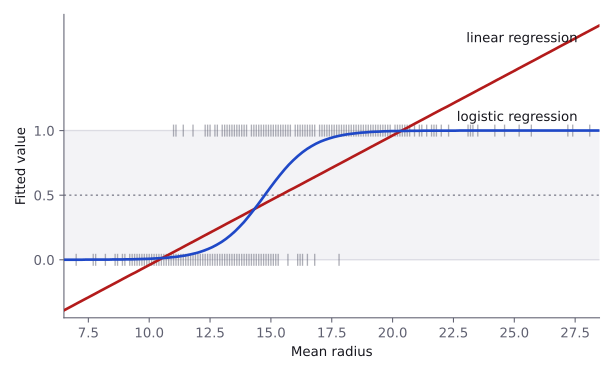
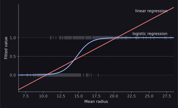
We want to keep the useful weighted score while turning it into a valid probability. That is the sigmoid's job.
The sigmoid function
Three values capture its main behaviour:
| Score | |||
|---|---|---|---|
| 0.119 | 0.500 | 0.881 |
- A very negative score becomes a probability close to 0.
- A score of 0 becomes exactly 0.5.
- A very positive score becomes a probability close to 1.
The sigmoid does not decide the class. It first converts the model's score into a probability. A threshold is applied later to turn that probability into a class.
OptionalOptional mathematics: properties of the sigmoid
We recommend going through this explanation after you understand the main role of the sigmoid. The linked Khan Academy lesson is also recommended if you want to see the calculus developed step by step.
The sigmoid is symmetric around :
Its derivative has a convenient form:
The derivative is largest, 0.25, at . The curve therefore changes fastest around probability 0.5 and flattens near 0 and 1.
One mathematical route to this curve begins with the differential equation
Its nonconstant solutions are . Requiring gives and produces the sigmoid. This is not something you need to derive to use the model. Khan Academy's Logistic models with differential equations develops this route in full.
The logistic regression model
The model has two steps:
Here is the estimated probability of class 1:
For example, if the weighted score is , then
The model is estimating an 88.1% probability of class 1. The score is also called the logit or decision score.
From a probability to a class
The usual rule for binary classification is
Because when , this is the same as checking the sign of the score. The points where
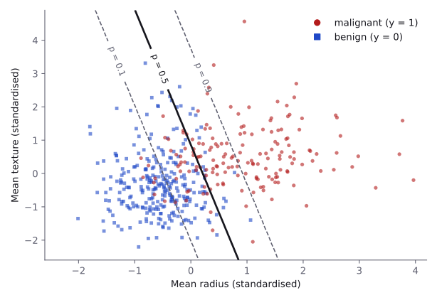
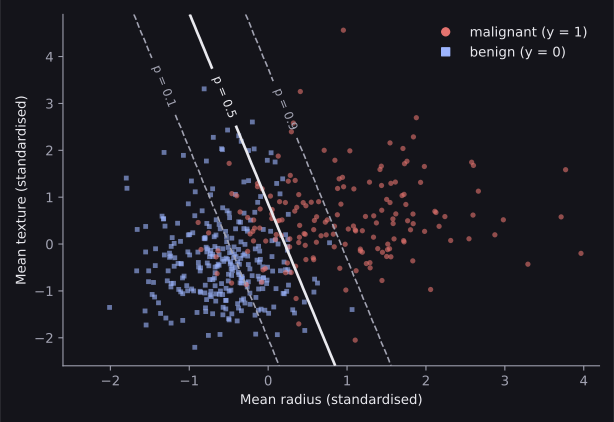
form the decision boundary. With one feature, the boundary is one cutoff point. With two features, it is a straight line. With many features, it is a flat surface called a hyperplane.
The probability curve is S-shaped, but the decision boundary is linear. Logistic regression is therefore a linear classifier.
The threshold does not have to be 0.5
The 0.5 threshold is a default, not a law. If missing a positive case is especially costly, we can lower the threshold. This usually detects more positive cases but also creates more false positives.
For example, a tumour model could predict class 1 whenever . The model's probabilities have not changed; only the rule that turns them into classes has changed. Model Evaluation Metrics explains how this affects precision, recall, ROC curves and other metrics.
Using LogisticRegression in practice
The practical workflow is much like linear regression: split the data, fit on the training part, and evaluate on data the model has not seen. stratify=y keeps roughly the same class proportions in both parts.
from sklearn.linear_model import LogisticRegression
from sklearn.model_selection import train_test_split
from sklearn.pipeline import make_pipeline
from sklearn.preprocessing import StandardScaler

X_train, X_test, y_train, y_test = train_test_split(
    X, y, test_size=0.2, stratify=y, random_state=0
)

model = make_pipeline(
    StandardScaler(),
    LogisticRegression(),
)
model.fit(X_train, y_train)

scores = model.decision_function(X_test)
probabilities = model.predict_proba(X_test)
predictions = model.predict(X_test)
The three prediction methods show each stage of the model:
decision_function → weighted scores z
predict_proba      → probabilities for classes 0 and 1
predict            → final classes after the default threshold
For a binary model, predict_proba returns two columns. Column 0 contains and column 1 contains .
print(scores[:3].round(2))
print(probabilities[:3].round(3))
print(predictions[:3])
The fitted weights and intercept are inside the last pipeline step:
clf = model[-1]
print(clf.classes_)          # [0 1]
print(clf.coef_.shape)       # (1, 30)
print(clf.intercept_.shape)  # (1,)

Z_test = model[:-1].transform(X_test)
print(np.allclose(scores, Z_test @ clf.coef_[0] + clf.intercept_))
print(np.allclose(probabilities[:, 1], 1 / (1 + np.exp(-scores))))
print(np.array_equal(predictions, (scores > 0).astype(int)))
# True
# True
# True
coef_ stores the weights, intercept_ stores the bias, and the checks confirm that scikit-learn follows the same score → sigmoid → class chain.
Evaluating predictions on unseen data
Accuracy is the fraction of examples classified correctly:
from sklearn.metrics import accuracy_score

accuracy = accuracy_score(y_test, predictions)
print(round(accuracy, 3))  # 0.974
This means the model classifies 97.4% of the held-out tumours correctly. Accuracy is a useful starting point, but it can be misleading when one class is much more common or when one kind of mistake matters more.
The Model Evaluation Metrics module covers confusion matrices, precision, recall, F1 and ROC AUC. Always use the metric named by the task. If a competition uses log loss or ROC AUC, the probabilities matter—not only the final classes.
Learning from probabilities: log loss
We now know what the model predicts. The next question is how it chooses and .
Linear regression minimises squared error. For classification, we instead want the model to give a high probability to the correct class and a low probability to the wrong class. Logistic regression measures this with log loss, also called binary cross-entropy or BCE.
For one example:
The combined formula for examples is
For a true class-1 example, the loss behaves like this:
| Predicted probability | 0.99 | 0.90 | 0.50 | 0.10 | 0.01 |
|---|---|---|---|---|---|
| Loss | 0.010 | 0.105 | 0.693 | 2.303 | 4.605 |
A confident correct prediction has almost no loss. A confident wrong prediction has a very large loss. Log loss especially punishes predictions that are confidently wrong. Training logistic regression means finding the weights and intercept that minimise the average log loss.
from sklearn.metrics import log_loss

y_true = [1, 0, 1]
p_hat = [0.9, 0.2, 0.6]
by_hand = -np.mean(np.log([0.9, 1 - 0.2, 0.6]))
print(round(by_hand, 4), round(log_loss(y_true, p_hat), 4))
# 0.2798 0.2798
Loss Functions compares log loss with other classification losses.
OptionalOptional mathematics: where log loss comes from
Suppose three labels are and the model predicts class-1 probabilities of . The probabilities assigned to the labels that actually occurred are
Assuming the samples are independent, the probability assigned to seeing all three labels is their product:
This product is called the likelihood. Training should make it as large as possible. Taking the logarithm turns the product into a sum, negating it turns maximisation into minimisation, and dividing by the number of samples gives log loss.
OptionalOptional mathematics: why not squared error?
Squared error can technically be combined with a sigmoid, but it gives less helpful optimisation behaviour. Its derivative with respect to is
For and a confidently wrong , this derivative is only about , so the model barely corrects one of its worst mistakes. Log loss gives the much stronger correction . Log loss also produces a convex objective for ordinary logistic regression, while squared error with a sigmoid does not.
Why scaling is a good default
LogisticRegression uses an iterative solver. When numeric features have very different ranges, the solver can take much longer to find good weights.
In the Breast Cancer dataset, mean smoothness lies roughly between 0.05 and 0.16, while mean area ranges from 143.5 to 2,501. Compare fitting the raw features with fitting standardised features:
raw = LogisticRegression().fit(X_train, y_train)
print(raw.n_iter_)  # [100], with a ConvergenceWarning

model = make_pipeline(StandardScaler(), LogisticRegression())
model.fit(X_train, y_train)
print(model[-1].n_iter_)            # [18]
print(model.score(X_test, y_test))  # 0.9736842105263158
On the raw features, the default solver reaches its 100-iteration limit and reports a ConvergenceWarning. With a much larger limit it can need roughly 3,000 iterations, depending on the library version. On standardised features, it converges in about 18.
For ordinary numeric tabular features, StandardScaler() followed by LogisticRegression() is therefore a good default. Scaling also makes weight magnitudes more comparable.
Interpreting the weights
The sign of a weight tells us which way that feature moves the prediction:
- a positive weight pushes the score and the probability towards class 1;
- a negative weight pushes them towards class 0; and
- a larger absolute weight changes the score more strongly, provided the feature scales are comparable.
As in linear regression, raw weight sizes should not be compared when features use different units. Correlated features also share credit in unstable ways. In the Breast Cancer data, mean radius has a correlation of 0.9979 with mean perimeter and 0.9874 with mean area. A model that includes all three can make stable predictions even when their individual weights change from one fit to another.
OptionalOptional mathematics: odds and log-odds
The odds of an event with probability are . A probability of 0.8 has odds of 4, often read as "4 to 1". A probability of 0.5 has odds of 1.
Solving for gives
Logistic regression is therefore linear in the log-odds. Increasing feature by one unit, while the others stay fixed, adds to the log-odds and multiplies the odds by .
log_reg = LogisticRegression()
log_reg.fit(radius, y)
w = log_reg.coef_[0, 0]
b = log_reg.intercept_[0]
print(round(w, 3), round(b, 2))  # 1.025 -15.13
print(round(np.exp(w), 2))       # 2.79

new = pd.DataFrame({"mean radius": [14.0, 15.0, 16.0]})
p = log_reg.predict_proba(new)[:, 1]
print(p.round(3))                # [0.316 0.562 0.782]
print((p / (1 - p)).round(3))    # [0.461 1.285 3.582]
print(round(-b / w, 2))          # 14.76
Each additional unit of mean radius multiplies the odds of malignancy by . The probability itself does not rise by a fixed amount because the sigmoid flattens near 0 and 1.
Where a linear boundary fails
Logistic regression separates classes with the boundary
No straight line can separate two concentric circles. Plain logistic regression therefore fails on this kind of data:
from sklearn.datasets import make_circles
from sklearn.model_selection import cross_val_score

X_c, y_c = make_circles(
    n_samples=500, noise=0.1, factor=0.5, random_state=0
)
plain = LogisticRegression()
print(round(cross_val_score(plain, X_c, y_c, cv=5).mean(), 3))
# 0.444
Creating better features
The feature-engineering idea from linear regression works here too. Starting with and , create
The classifier is still linear in these new features, but its boundary can now be curved in the original two-dimensional space.
from sklearn.preprocessing import PolynomialFeatures

quadratic = make_pipeline(
    PolynomialFeatures(degree=2),
    StandardScaler(),
    LogisticRegression(),
)
print(round(cross_val_score(quadratic, X_c, y_c, cv=5).mean(), 3))
# 0.988
Accuracy rises from 0.444 to 0.988. Feature engineering changes the decision boundaries that a linear classifier can represent. If useful features are hard to design, a naturally non-linear model such as a decision tree may be a better choice.
More than two classes
Binary logistic regression uses one score and the sigmoid. For classes, multinomial logistic regression computes one score per class:
The softmax function turns all scores into probabilities:
Every probability is between 0 and 1, all of them add to 1, and the class with the largest probability is predicted. For two classes, softmax reduces to a sigmoid applied to the difference between the two scores.
from sklearn.datasets import load_iris

X_iris, y_iris = load_iris(return_X_y=True)
iris_model = make_pipeline(StandardScaler(), LogisticRegression())
iris_model.fit(X_iris, y_iris)

print(iris_model[-1].coef_.shape)  # (3, 4): one row per class
z = iris_model.decision_function(X_iris[:2])
p_softmax = np.exp(z) / np.exp(z).sum(axis=1, keepdims=True)
print(np.allclose(p_softmax, iris_model.predict_proba(X_iris[:2])))
# True
The model is trained with multi-class log loss,
which penalises a low probability for the correct class. With the default solver, scikit-learn 1.9.1 fits this multinomial model for three or more classes; the former multi_class parameter no longer exists.
OptionalOptional: one-vs-rest
Another approach trains one binary classifier per class: class 0 against everything else, class 1 against everything else, and so on. This is called one-vs-rest, and the class whose classifier gives the highest score is predicted.
from sklearn.datasets import load_wine
from sklearn.multiclass import OneVsRestClassifier

for load in (load_iris, load_wine):
    X_d, y_d = load(return_X_y=True)
    for estimator in (
        LogisticRegression(),
        OneVsRestClassifier(LogisticRegression()),
    ):
        pipe = make_pipeline(StandardScaler(), estimator)
        accuracy = cross_val_score(pipe, X_d, y_d, cv=5).mean()
        print(load.__name__, type(estimator).__name__, round(accuracy, 3))
# load_iris LogisticRegression 0.960
# load_iris OneVsRestClassifier 0.927
# load_wine LogisticRegression 0.983
# load_wine OneVsRestClassifier 0.989
Neither approach wins on every dataset. The multinomial model is the usual starting point because it learns one consistent set of probabilities. The "liblinear" solver handles multiclass data only when wrapped in OneVsRestClassifier.
How the model learns its weights
Unlike ordinary least squares, logistic regression has no simple closed-form formula for its best weights. An iterative optimiser follows this loop:
start with weights
→ calculate scores and probabilities
→ calculate log loss
→ update the weights
→ repeat until the loss stops improving
Gradient descent and related optimisers are covered properly in Gradient Descent. For this module, the important point is that fit repeats these steps until the weights settle or max_iter is reached.
OptionalOptional mathematics: the gradient
For one sample, combining the derivative of the sigmoid with log loss gives the useful result
The full gradients are
The log-loss objective for ordinary logistic regression is convex, so it has no poor local minimum separate from the best one. With an appropriate optimiser, training can approach the same best solution from different starting points.
Useful LogisticRegression settings
These are the settings a beginner is most likely to need:
| Setting | Default | Meaning |
|---|---|---|
solver |
"lbfgs" |
Algorithm used to fit the weights |
max_iter |
100 |
Maximum fitting iterations |
tol |
0.0001 |
Threshold for stopping |
class_weight |
None |
Importance assigned to each class |
fit_intercept |
True |
Whether to learn the bias |
Setting class_weight="balanced" automatically weights classes according to how often they appear.
Where logistic regression is useful
- Tabular classification: a standardised logistic regression is a fast, strong baseline. Its 0.974 test accuracy on the Breast Cancer split is a demanding result for a more complicated model to beat.
- Precomputed features: a pretrained model can turn images, text or audio into embedding vectors. Logistic regression on those vectors is often called a linear probe.
- Problems with useful engineered features: polynomial or hand-designed features can let the model represent boundaries it could not express from the raw inputs.
When the classes need a boundary that useful features cannot make linear, try a naturally non-linear model.
Logistic regression in olympiad tasks
This example shows that logistic regression is not only a simple tabular model. It is also useful on top of powerful learned representations.
The whole idea in one view
prediction:      features → weighted score z → sigmoid → probability
                 probability → threshold → class

training:        probabilities → log loss → iterative optimiser
                 → learned weights

generalisation:  train on one part → evaluate on unseen data

improvement:     slow fitting → scale numeric features
                 curved boundary → engineer features or change model
                 multiple classes → softmax
The central idea is still the one from linear regression: learn a weighted combination of features. Logistic regression adds the sigmoid so that the result becomes a probability, then uses a threshold to turn that probability into a class.
Resources
| Source | Title | Why read it |
|---|---|---|
| scikit-learn | User Guide: Logistic regression | The sections 'Binary Case', 'Multinomial Case' and 'Solvers' explain the model and its optimisation algorithms. |
| scikit-learn | LogisticRegression | The complete API reference for the estimator and its settings. |
| Google for Developers | Logistic regression: Calculating a probability with the sigmoid function | The section 'Transforming linear output using the sigmoid function' shows the step from a linear score to a probability. |
| Google for Developers | Logistic regression: Loss and regularization | The section 'Log Loss' explains why classification uses a different loss from linear regression. |
| Khan Academy | Logistic models with differential equations | An optional calculus-based route to the logistic function, including the differential equation it solves. |
| James, Witten, Hastie, Tibshirani | An Introduction to Statistical Learning | A free textbook. Its chapter on classification treats logistic regression with more statistical depth. |
Practice problems
| Solved | Source | Problem | Difficulty | Tags |
|---|---|---|---|---|
| Kaggle | Titanic | Easy | binary classification, tabular | |
| IOAI 2026 | Ghost of the Machine | Hard | nlp, embeddings |
Finished this module? Mark it done.
Comments
Stuck on something, spotted a mistake, or found a resource that helped you? Tell us below.
Loading comments