5Deep Learning 5.2Deep Learning Fundamentals
5.2.2 Gradient Descent
How a model improves its weights one small step at a time: the update rule, the learning rate, mini-batches, and the optimisers PyTorch gives you.
Why gradient descent?
In Multi-Layer Perceptrons, we built networks out of layers of weights and biases. We did not say how a network finds good values for them. That is the job of gradient descent, and it is the reason the training loop from PyTorch Basics works at all: every call to optimizer.step() is one step of gradient descent.
For some models there is a shortcut. Linear Regression has a formula that gives the best weights directly. A neural network has no such formula, so we find its weights the way you would walk down a hill in thick fog: feel which way the ground slopes, take a small step downhill, and repeat.
This module explains that idea properly, first with one weight you can follow by hand, then with real data, and then with the optimisers PyTorch gives you. How the slope is actually computed for every weight in a deep network is the topic of the next module, Backpropagation.
What you need to know
By the end of this module, you should be comfortable with these ideas:
| Idea | In one line |
|---|---|
| Loss surface | The loss seen as a landscape over all possible weight values; training looks for its lowest point. |
| Gradient | The direction in which the loss rises fastest; its negative points downhill. |
| Update rule | New weight = old weight − learning rate × gradient. |
| Learning rate | How big each step is. Too small is slow, too large overshoots and can blow up. |
| Feature scaling | Features on similar scales make the landscape easier to walk down. |
| Batch, stochastic and mini-batch | Whether each step uses all the data, one sample, or a small group. |
| Epoch, iteration, batch size | One pass over the data; one update step; how many samples each step uses. |
| Momentum and Adam | Improved versions of the basic step that most real training uses. |
Learn it properly
This page walks you through the ideas with code you can run, but a good explanation from another angle helps them stick. Pick one of the options below and come back to the walkthrough afterwards.
Pick one main course
One clear explanation, followed properly, is worth more than five half-watched videos. Start with our pick and use the others only if something does not click.
Our pick: 3Blue1Brown, then Google's Crash Course
Start with 3Blue1Brown's video Gradient descent, how neural networks learn. It shows the loss surface and the downhill steps moving, which a written page cannot. It is chapter 2 of a series; if you have not seen chapter 1, watch that first.
Then read the two short lessons in Google's Machine Learning Crash Course: Gradient descent and Hyperparameters. They also start from a linear model, as this page does, and their interactive exercises let you watch different learning rates succeed and fail.
If you prefer something else
- Course notes: Stanford's CS231n notes on optimisation explain the loss surface, numerical and analytic gradients, and mini-batches in one page.
- A textbook: chapter 12 of Dive into Deep Learning covers gradient descent, SGD, mini-batches, momentum and Adam with more maths than you need right now. It is a good second read.
- Later, for optimisers: Sebastian Ruder's overview of gradient descent optimisation algorithms compares momentum, Adam and many others. You do not need it at this level, but it is the place to go when you want to know why Adam behaves as it does.
A quick tour
The rest of this page shows gradient descent at work, from one weight to real data to PyTorch. Go through your chosen resource first if the idea is completely new, then follow the code here in a notebook and change the numbers to see what happens.
Walking downhill
A model's loss depends on its weights. If we could draw the loss for every possible value of the weights, we would get a landscape: the loss surface. Good weights sit at the bottom of a valley. We cannot see the whole landscape, because a real network has millions of weights, but at the point where we stand we can work out one thing: the slope.

The rest of this section turns that picture into one line of maths.
For a single weight , the slope is the derivative . If it is positive, the loss goes up as grows, so we should make smaller. If it is negative, we should make bigger. Either way, we move in the direction opposite to the slope:
The Greek letter ("eta") is the learning rate: a small positive number that sets how big each step is. The arrow means "replace with". That one line is gradient descent.
One weight, worked by hand
Let us take the simplest loss we can: . Its lowest point is obviously at , which lets us check that the method finds it. The slope is .
Start at with a learning rate of :
- The slope at is . It is negative, so we move right: .
- The slope at is , so .
The same steps in code, five times:
w = 0.0              # our starting guess
learning_rate = 0.1

for step in range(1, 6):
    slope = 2 * (w - 3)                 # dL/dw at the current w
    w = w - learning_rate * slope       # one step downhill
print(step, round(w, 4))1 0.6
2 1.08
3 1.464
4 1.7712
5 2.017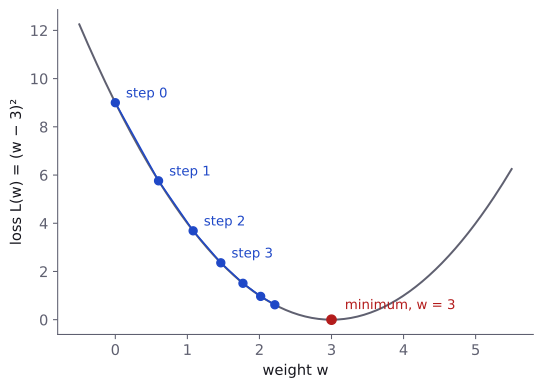
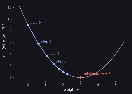
Notice two things. The steps get smaller by themselves, because the slope gets flatter near the bottom; we never had to tell the method to slow down. And we never jump straight to 3: gradient descent only ever takes small steps, and keeps going until the answer is close enough.
Many weights and the gradient
A real model has many weights, so the loss is a surface in many dimensions. For each weight we can ask the same question: if I nudge only this weight, does the loss go up or down, and how fast? The answer for weight is the partial derivative , and the list of all of them is the gradient, written ("nabla L"):
The gradient points in the direction in which the loss rises fastest, so we step the opposite way. Written for all the weights at once, the update rule becomes
With two weights we can still draw this, seen from above like a map. Contour lines join points with the same loss, the dark blue areas are the lowest, and every path follows the negative gradient downhill:
That is the whole algorithm. Everything else on this page is about doing it well: how big the steps should be, how much data to use for each step, and how to make the steps smarter.
Gradient descent on real data
Now we can fit a straight line to real data with gradient descent, and check the answer against the formula. We use the same data as Linear Regression: predicting the petal width of an iris flower from its petal length.
import numpy as np
from sklearn.datasets import load_iris

iris = load_iris()
petal_length = iris.data[:, 2]
petal_width = iris.data[:, 3]
The model is and the loss is the mean squared error, . Its two partial derivatives are
OptionalWhere these two derivatives come from
Take one sample and write its error as . Its squared error is .
By the chain rule, . Since , changing by a little changes by times that amount, so . Changing changes by exactly the same amount, so .
That gives and . The loss is the average of the squared errors, and the derivative of an average is the average of the derivatives, which gives the two formulas above. The next module turns this kind of chain-rule reasoning into a method that works for any network.
In code, each of those sums becomes an np.mean. The loop below is the update rule from earlier, now with two weights:
def gradient_descent(x, y, learning_rate, steps):
    w, b = 0.0, 0.0
    for step in range(steps):
        prediction = w * x + b
        error = prediction - y
        grad_w = 2 * np.mean(error * x)      # dL/dw
        grad_b = 2 * np.mean(error)          # dL/db
        w = w - learning_rate * grad_w
        b = b - learning_rate * grad_b
    return w, b

w, b = gradient_descent(petal_length, petal_width, 0.02, 2000)
print(round(w, 3), round(b, 3))0.416 -0.363Now let us compare with the exact answer. np.polyfit fits the best straight line directly, using the formula from Linear Regression:
slope, intercept = np.polyfit(petal_length, petal_width, 1)
print(round(slope, 3), round(intercept, 3))0.416 -0.363The same line, . Gradient descent needed 2,000 small steps to get there, where the formula needed none. For linear regression that makes gradient descent look pointless, but the formula only exists for a few simple models. For a neural network, the steps are the only way.
Choosing the learning rate
The learning rate is the setting you will change most often, so it is worth seeing what it does. Here is the loss over the first 60 steps of the iris fit for three learning rates:
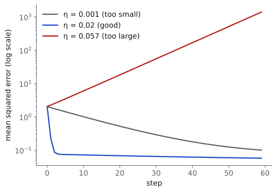
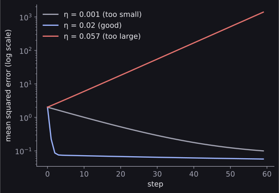
- Too small (): every step goes the right way, but the steps are tiny. After 60 steps the loss is still about 0.1, more than twice the best possible 0.042.
- About right (): the loss drops sharply in the first few steps, then keeps improving slowly.
- Too large (): each step jumps past the bottom of the valley and lands higher up on the other side. The error grows every step: after 60 steps the loss is above 1,000, and given enough steps it overflows to
infand thennan.
For this problem, anything above about 0.055 diverges. You will never know that number in advance for a real network, so in practice we try a few values that differ by a factor of 10 (0.1, 0.01, 0.001) and watch the loss curve. If the loss goes up or becomes nan, the rate is too large; if it barely moves, it is too small. Picking the rate carefully is part of Hyperparameter Tuning.
Why scaling the features helps
Look again at the blue curve: after its fast start, the loss improves very slowly. The reason is the shape of the valley. Petal lengths run from 1 to 7, so the loss changes much faster when we change than when we change . The valley is long and narrow, and a step size that is safe for the steep direction is tiny for the flat one.
Standardising the feature (subtracting its mean and dividing by its standard deviation) makes the valley round, so both directions can use the same step size. Let us count how many steps each version needs to get within of the best possible loss:
def steps_to_converge(x, y, learning_rate, target_loss):
    w, b = 0.0, 0.0
    for step in range(10_000):
        error = w * x + b - y
        if np.mean(error ** 2) < target_loss:
            return step
        w = w - learning_rate * 2 * np.mean(error * x)
        b = b - learning_rate * 2 * np.mean(error)

best_line = slope * petal_length + intercept
best_loss = np.mean((best_line - petal_width) ** 2)
target = best_loss + 1e-6

length_mean = petal_length.mean()
length_std = petal_length.std()
scaled_length = (petal_length - length_mean) / length_std

print(steps_to_converge(petal_length, petal_width, 0.02, target))
print(steps_to_converge(scaled_length, petal_width, 0.1, target))758
33The scaled version gets there in 33 steps instead of 758, and it tolerates a larger learning rate too. This is why neural networks almost always get scaled inputs; Scaling in Scikit-learn Basics shows how to do it without leaking information from the test data. (The weight learned on scaled data is in "per standard deviation" units, so it is not 0.416 any more, but the predictions are the same line.)
Batches, epochs and iterations
So far, every step used all 150 flowers to compute the gradient. That is batch gradient descent. With a million training images it would be far too slow: one step would mean running the whole dataset through the network. There are three options:
| Method | Data used for one step | Trade-off |
|---|---|---|
| Batch gradient descent | The whole training set | Accurate gradient, but each step is slow |
| Stochastic gradient descent (SGD) | One sample | Very fast steps, but each gradient is very noisy |
| Mini-batch gradient descent | A small group, such as 32 samples | The usual choice: fast steps with a reasonable gradient |
The animation shows what a noisy gradient does. Each step uses a random part of the data, so the paths wobble, but on average they still head for the minimum:
Confusingly, people and libraries say "SGD" for mini-batch gradient descent too; PyTorch's torch.optim.SGD is used with mini-batches almost always. The vocabulary you will meet everywhere:
- Batch size: how many samples go into each step.
- Iteration: one update step, using one mini-batch.
- Epoch: one full pass over the training data. With 150 samples and a batch size of 16, one epoch is 10 iterations (nine batches of 16 and a last one of 6).
Here is mini-batch gradient descent on the iris data. The data is shuffled at the start of every epoch, so the batches are different each time:
rng = np.random.default_rng(0)
w, b = 0.0, 0.0
learning_rate = 0.02
batch_size = 16

for epoch in range(100):
    order = rng.permutation(len(petal_length))    # shuffle
    for start in range(0, len(order), batch_size):
        batch = order[start:start + batch_size]
        x_batch = petal_length[batch]
        y_batch = petal_width[batch]
        error = w * x_batch + b - y_batch
        w = w - learning_rate * 2 * np.mean(error * x_batch)
        b = b - learning_rate * 2 * np.mean(error)

print(round(w, 3), round(b, 3))0.418 -0.365Close to the best line, but not exactly on it. Each mini-batch gives a slightly different gradient, so the weights keep jiggling around the bottom of the valley instead of settling. In practice this noise is harmless and even useful, and the speed is worth it.
Shuffling matters more than it looks. The iris data is sorted by species; without shuffling, each mini-batch would contain only one kind of flower, and every step would pull the line towards that species alone.
Momentum and Adam
Plain gradient descent has two weaknesses you have now seen: it crawls along long, flat valleys, and it zigzags across narrow ones. Two improvements fix most of this, and you will use them far more often than the plain version.
Momentum keeps a running "velocity": each step adds the new gradient to a fraction (usually 0.9) of the previous step.
Directions that stay consistent build up speed, like a ball rolling downhill, while zigzags cancel out.
Adam goes further. It keeps running averages of both the gradients and their squares for every weight, and uses them to give each weight its own step size. Weights with small, steady gradients get relatively bigger steps, and weights with large, jumpy ones get smaller steps. You do not need its exact formula yet; the d2l.ai chapter on Adam has it when you want it.
In PyTorch, switching between them is one line. Here is the same iris fit with each, 100 steps each:
import torch
from torch import nn

X = torch.tensor(petal_length, dtype=torch.float32).reshape(-1, 1)
Y = torch.tensor(petal_width, dtype=torch.float32).reshape(-1, 1)

def train(optimizer_name, steps=100):
    torch.manual_seed(0)
    model = nn.Linear(1, 1)
    params = model.parameters()
    if optimizer_name == "SGD":
        optimizer = torch.optim.SGD(params, lr=0.02)
    elif optimizer_name == "SGD with momentum":
        optimizer = torch.optim.SGD(params, lr=0.02, momentum=0.9)
    else:
        optimizer = torch.optim.Adam(params, lr=0.1)
    loss_fn = nn.MSELoss()
    for step in range(steps):
        loss = loss_fn(model(X), Y)
        optimizer.zero_grad()
        loss.backward()
        optimizer.step()
    return loss.item()

for name in ["SGD", "SGD with momentum", "Adam"]:
print(name, round(train(name), 4))SGD 0.0833
SGD with momentum 0.0421
Adam 0.0421After 100 steps, plain SGD is still twice as far from the best loss (0.042) as the other two, which have essentially reached it. The training loop is exactly the five steps from PyTorch Basics; only the optimiser changed.
Which should you use? For neural networks, Adam is the usual first choice, and PyTorch's default Adam learning rate of 0.001 is a sensible starting point. SGD with momentum is the other common choice. The torch.optim documentation lists the others.
What you can ignore for now
A few topics come up in every discussion of gradient descent. You will meet them later; none of them should worry you yet.
- Local minima and saddle points. A network's loss surface is not one neat valley, so in principle gradient descent could get stuck in a dip that is not the lowest point, or on a flat saddle. For linear regression this cannot happen, because its loss surface has exactly one valley. For neural networks it matters much less in practice than it sounds, and mini-batch noise and momentum help push past flat regions.
- Learning-rate schedules, which lower the learning rate as training goes on, and weight decay, which gently pulls weights towards zero. Both are Silver-level refinements.
- Second-order methods such as Newton's method, which use the curvature of the loss as well as its slope. They are too expensive for large networks.
Common mistakes
| Mistake | What you see | Fix |
|---|---|---|
| Learning rate too large | The loss rises, jumps around, or becomes inf or nan |
Divide the learning rate by 10 and try again. |
| Learning rate too small | The loss falls so slowly it looks stuck | Multiply it by 10, and check the loss curve over more steps. |
| Features on very different scales | Slow progress after a fast start, or instability with any useful learning rate | Standardise the inputs. |
| Not shuffling sorted data | Training that swings between classes and never settles | Shuffle every epoch (a PyTorch DataLoader does it with shuffle=True). |
| Judging progress by one mini-batch | A loss that jumps up and down from step to step | Look at the average loss over a whole epoch. |
Forgetting optimizer.zero_grad() in PyTorch |
No error, but gradients from every step add up and training misbehaves | Clear the gradients before each backward(); Backpropagation explains why they add up. |
How to practise
- Do the interactive exercises in Google's Gradient descent and Hyperparameters lessons.
- Change the numbers in this page's code: try learning rates between 0.001 and 0.06 on the iris fit, and batch sizes of 1, 16 and 150, and predict what the result will be before you run it.
- Write gradient descent for logistic regression yourself, using the gradient given in that module, and compare your weights with scikit-learn's.
There are no gradient-descent problems on CodeChef, CS50 or HackerRank, so these exercises are the practice for this module.
Check yourself
What comes next
Gradient descent needs the gradient of the loss with respect to every weight. For a straight line we could work it out by hand; for a network with millions of weights we need a systematic method.
- Backpropagation: how the gradient is computed for every weight in a network, and what PyTorch's
backward()does for you.
Resources
| Source | Title | Why read it |
|---|---|---|
| 3Blue1Brown | Gradient descent, how neural networks learn | Our recommended starting point. A visual explanation of the whole idea in one video. |
| Machine Learning Crash Course: Gradient descent | Short written lessons with interactive exercises. Read it together with the next page on hyperparameters. | |
| Machine Learning Crash Course: Hyperparameters | Learning rate, batch size and epochs, with pictures of what goes wrong. | |
| Stanford CS231n | Optimization: Stochastic Gradient Descent | Course notes that connect the loss surface, gradients and mini-batches. |
| d2l.ai | Dive into Deep Learning, chapter 12: Optimization Algorithms | The maths behind gradient descent, SGD, mini-batches, momentum and Adam, with code. |
| Sebastian Ruder | An overview of gradient descent optimization algorithms | A well-known survey of momentum, Adam and the rest. Read it later, once the basics are clear. |
| PyTorch | torch.optim | The reference for PyTorch's optimisers and their settings. |
Finished this module? Mark it done.
Comments
Stuck on something, spotted a mistake, or found a resource that helped you? Tell us below.
Loading comments