5Deep Learning 5.2Deep Learning Fundamentals
5.2.1 Multi-Layer Perceptrons
Build up a neural network from a single neuron: layers, the forward pass as matrix maths, why the nonlinearity matters, and an MLP in PyTorch.
Why learn multi-layer perceptrons?
In PyTorch Basics, we trained a single straight line: one weight and one bias. In Logistic Regression, we saw the same idea with a sigmoid on top, which draws one straight boundary between two classes. Both are useful, but both have the same limit: they can only draw straight lines (or flat planes, with more features).
The classic example is XOR, short for "exclusive or". It takes two inputs, each 0 or 1, and outputs 1 when exactly one of them is 1:
| XOR | ||
|---|---|---|
| 0 | 0 | 0 |
| 0 | 1 | 1 |
| 1 | 0 | 1 |
| 1 | 1 | 0 |
Put the four inputs on the corners of a square and try to draw one straight line with both 1s on one side and both 0s on the other. You cannot: the 1s sit on opposite corners, and so do the 0s. Wherever the line goes, at least one point ends up on the wrong side, so logistic regression can never get all four right, however long it trains.
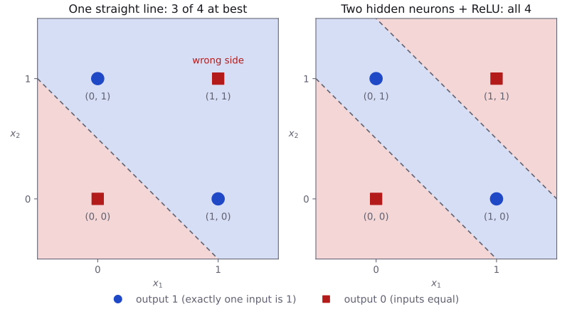
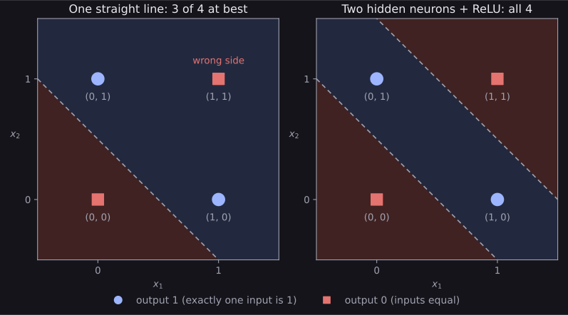
A multi-layer perceptron (MLP) removes that limit. It stacks many small units, called neurons, into layers, and puts a simple bend, called an activation function, between the layers. The result can learn curved and even patchy boundaries that no single line could draw. For XOR, two hidden neurons are already enough; we build that exact network by hand in Why the activation function matters.
MLPs matter for IOAI in two ways. First, they are a solid model on their own for tabular data and for embeddings produced by other models. Second, every bigger network you will meet later, such as the convolutional networks in Convolutional Neural Networks, ends with MLP layers and is trained in exactly the same way. If you understand an MLP, the rest of deep learning is variations on it.
What you need to know
By the end of this module, you should be comfortable with these ideas:
| Idea | In one line |
|---|---|
| Neuron | A weighted sum of the inputs, plus a bias, passed through an activation function. |
| Layer | Many neurons that all read the same inputs; in code, one matrix multiplication. |
| Hidden layer | A layer between the input and the output, whose values nobody labels. |
| Width and depth | How many neurons a layer has, and how many layers there are. |
| Forward pass | Running inputs through the layers, one after another, to get the output. |
| Parameters | All the weights and biases; what training changes. |
| Why activations matter | Without them, any stack of layers collapses into a single linear layer. |
nn.Sequential and nn.Module |
The two usual ways to write an MLP in PyTorch. |
How the network learns its parameters is the subject of the next three modules. Here we only need the big picture of training, and we will say clearly where each detail is covered.
Learn it properly
This page walks you through the ideas with small, runnable examples. A good course gives you the pictures and the practice that make them stick, so use both.
Pick one main course
As in the earlier modules, choose one main resource and finish it rather than sampling several.
Our pick: 3Blue1Brown
Start with 3Blue1Brown's But what is a neural network?, the first chapter of a short deep learning series. In under 20 minutes it shows what neurons, layers, weights and biases are, using a network that reads handwritten digits. The pictures in it are exactly the ones worth having in your head while you read this page.
The later chapters of the series cover gradient descent and backpropagation. You can watch them now or wait until Gradient Descent and Backpropagation, which link back to them.
If you prefer something else
- A free book: chapter 1 of Michael Nielsen's Neural Networks and Deep Learning builds the same digit network with the maths written out. It uses plain Python and NumPy rather than PyTorch, but the ideas carry over directly.
- A textbook with PyTorch code: the Multilayer Perceptrons section of Dive into Deep Learning uses the same matrix notation as this page.
- Course notes: Stanford CS231n's Setting up the Architecture is short and precise, with a good section on counting parameters.
- Play with it: the TensorFlow Playground trains a small MLP in your browser. Try adding and removing hidden neurons and watch the boundary change. (Only the website uses TensorFlow; you do not need it for anything else.)
A quick tour
The rest of this page builds an MLP one piece at a time: first a single neuron, then a layer, then a stack of layers, and finally a small network that solves a problem a straight line cannot. Every code cell runs as written, so type them into a notebook as you go.
From logistic regression to a neuron
A neuron does two things. It takes a weighted sum of its inputs and adds a bias, and then it passes the result through an activation function. For an input with features, weights and bias :
If the activation is the sigmoid, this is exactly logistic regression: one neuron is a logistic regression model. Let us compute one by hand:
import torch

x = torch.tensor([2.0, 1.0, 3.0])     # one sample with 3 features
w = torch.tensor([0.5, -1.0, 0.25])   # one weight per feature
b = torch.tensor(0.1)                 # the bias

z = torch.dot(w, x) + b               # 1.0 - 1.0 + 0.75 + 0.1
a = torch.sigmoid(z)                  # the activation
print(z, a)tensor(0.8500) tensor(0.7006)The weighted sum is , and the sigmoid squashes it to . Each weight says how much its feature pushes the output up (positive weight) or down (negative weight), and the bias shifts the whole sum. The numbers and are the neuron's parameters: the things training will learn.
The sigmoid is only one choice of activation. Modern networks mostly use others, such as ReLU, which we will use below; Activation Functions compares them. For this module, all you need is that the activation is a fixed, nonlinear function applied to each number.
A layer of neurons
A layer is many neurons side by side, all reading the same inputs, each with its own weights and bias. If we stack each neuron's weights as one row of a matrix , the whole layer becomes one matrix multiplication.
We also process many samples at once, a batch. With the samples as the rows of a matrix (one row per sample), a layer with neurons computes
where has shape for samples with features, has shape , and has entries, one per neuron. The result has shape : one row per sample, one column per neuron. Tensors, Matrices, and Related Mathematical Functions goes through these shape rules carefully; here we just check them in code:
torch.manual_seed(0)
X = torch.tensor([[2.0, 1.0, 3.0],
                  [0.0, 1.0, 0.0],
                  [1.0, 2.0, 1.0],
                  [4.0, 0.0, 1.0]])   # 4 samples, 3 features
W = torch.randn(2, 3)                 # 2 neurons, 3 weights each
b = torch.zeros(2)                    # one bias per neuron

Z = X @ W.T + b                       # (4, 3) @ (3, 2) -> (4, 2)
Z.shapetorch.Size([4, 2])PyTorch packages exactly this as nn.Linear(in_features, out_features). It stores the weights with the same shape as our W, one row per neuron:
from torch import nn

layer = nn.Linear(3, 2)               # 3 inputs, 2 neurons
layer.weight.shape, layer.bias.shape(torch.Size([2, 3]), torch.Size([2]))Calling the layer does the multiplication for us. We can confirm that it matches the formula:
by_hand = X @ layer.weight.T + layer.bias
torch.allclose(layer(X), by_hand)Truetorch.allclose checks that two tensors are equal up to tiny rounding differences. Notice that nn.Linear starts with random weights; training will replace them with useful ones.
Stacking layers: the forward pass
An MLP chains layers together. The output of one layer, after its activation, becomes the input of the next. With two layers and the ReLU activation, the forward pass for a batch is
- is the input layer: just the data, with no parameters.
- is a hidden layer. Its values are features the network invents for itself; nobody labels them, which is why it is called hidden.
- is the output layer: one number per output, such as one score per class.
The number of neurons in a layer is its width, and the number of layers with parameters is the network's depth. The network above has depth 2. (Counting conventions differ between books, so do not worry if one calls this network "two-layer" and another "three-layer"; what matters is how many weight matrices it has.)
In PyTorch, nn.Sequential runs its parts one after another, which is exactly a forward pass. This MLP takes 4 features, has one hidden layer of 16 neurons, and outputs 3 scores, for example one per class of a three-class problem:
model = nn.Sequential(
    nn.Linear(4, 16),    # input (4 features) -> 16 hidden neurons
    nn.ReLU(),           # the activation, applied to each number
    nn.Linear(16, 3),    # 16 hidden neurons -> 3 output scores
)
The output layer has no activation here. That is deliberate: raw scores, called logits, are what PyTorch's classification losses expect. Loss Functions explains why.
Counting parameters
A layer from inputs to neurons has weights and biases, so parameters. For the model above, that is for the first layer and for the second, 131 in total. We can let PyTorch count them:
n_params = 0
for p in model.parameters():          # every weight matrix and bias
    n_params += p.numel()             # numel = number of elements
n_params131Counting parameters is a quick sanity check. It tells you roughly how much the model can memorise, and in a contest it tells you whether a model will fit in memory and train in time. The ReLU contributes nothing to the count: activations have no parameters.
Why the activation function matters
It is tempting to drop the activations and stack plain linear layers. It does not work: two linear layers in a row are just one linear layer. Writing the two layers out,
which is a single layer with weights and bias . The same argument works for any number of layers, so without activations even a hundred layers can only draw a straight boundary, like logistic regression. Let us check it numerically:
first = nn.Linear(3, 5)
second = nn.Linear(5, 2)
two_layers = second(first(X))              # no activation in between

W_combined = second.weight @ first.weight  # (2, 5) @ (5, 3) -> (2, 3)
b_combined = second.weight @ first.bias + second.bias
one_layer = X @ W_combined.T + b_combined

torch.allclose(two_layers, one_layer, atol=1e-6)TrueThe nonlinear activation between the layers is what breaks this collapse and lets the network bend its boundary. That is the whole reason activations exist. Which activation to choose, and why ReLU became the default, is the topic of Activation Functions.
XOR, from the start of this page, shows the difference clearly. The activation we will use is ReLU, short for rectified linear unit: , so negative numbers become 0 and positive numbers pass through unchanged. Here is a network with two hidden neurons and one output, with weights chosen by hand rather than trained. It is the classic solution from section 6.1 of the free book Deep Learning by Goodfellow, Bengio and Courville.
xor_x = torch.tensor([[0.0, 0.0],
                      [0.0, 1.0],
                      [1.0, 0.0],
                      [1.0, 1.0]])   # one row per input
W1 = torch.tensor([[1.0, 1.0],
                   [1.0, 1.0]])      # 2 hidden neurons
b1 = torch.tensor([0.0, -1.0])
W2 = torch.tensor([[1.0, -2.0]])     # 1 output neuron
b2 = torch.tensor([0.0])

H = torch.relu(xor_x @ W1.T + b1)    # hidden layer, with ReLU
print(H)
print((H @ W2.T + b2).squeeze(1))    # (4, 1) -> (4,)

H_no_relu = xor_x @ W1.T + b1        # same weights, no ReLU
print((H_no_relu @ W2.T + b2).squeeze(1))tensor([[0., 0.],
[1., 0.],
[1., 0.],
[2., 1.]])
tensor([0., 1., 1., 0.])
tensor([2., 1., 1., 0.])Read the hidden values H one column at a time. The first neuron computes , which counts how many inputs are 1. The second computes , which is negative unless both inputs are 1, so the ReLU turns it into 0 everywhere except the last row. The output neuron takes the count and subtracts the second neuron twice: for the two middle rows, but for . That is exactly XOR: 0, 1, 1, 0.
Without the ReLU, the second neuron keeps its value of for the input , and the whole network collapses to the single linear formula , which gives 2, 1, 1, 0 instead. That is one straight line again, and no straight line can do XOR. The two hidden neurons are the two dashed lines in the right-hand picture at the top of this page; the ReLU is what lets the network combine them into a strip.
What training means
So far the weights are random, so the network's outputs are useless. Training adjusts all the parameters so that the outputs match the labels. It repeats the same five steps you saw in PyTorch Basics, and each step has its own module in this part of the guide:
- Forward pass: compute the outputs for a batch (this module).
- Loss: measure how wrong the outputs are with one number (Loss Functions).
- Clear old gradients.
- Backward pass: work out how the loss changes with each parameter, the gradients (Backpropagation).
- Update: move each parameter a small step against its gradient (Gradient Descent).
You do not need to understand steps 2, 4 and 5 in detail yet to follow the next example; PyTorch does them for you, and the next modules open each one up.
A problem a straight line cannot solve
Now let us put everything together on a problem where a linear model fails. We scatter 400 random points in the square from to , and label a point 1 when its two coordinates have the same sign (top right or bottom left) and 0 otherwise. This checkerboard of four quarters is a version of the classic XOR problem, and no single straight line can separate it.
torch.manual_seed(0)
points = torch.rand(400, 2) * 2 - 1   # 400 points in the square
x_coord = points[:, 0]
y_coord = points[:, 1]
same_sign = x_coord * y_coord > 0     # True when x and y share a sign
labels = same_sign.float()            # 1.0 or 0.0

train_x, test_x = points[:300], points[300:]
train_y, test_y = labels[:300], labels[300:]
train_x.shapetorch.Size([300, 2])We keep the last 100 points aside as a test set, so we can check the models on points they never saw. First, logistic regression, from Logistic Regression:
from sklearn.linear_model import LogisticRegression

linear = LogisticRegression()
linear.fit(train_x.numpy(), train_y.numpy())
round(linear.score(test_x.numpy(), test_y.numpy()), 2)0.58With two roughly equal classes, guessing gets about 0.5, so 0.58 means the straight line has learned almost nothing. Now a small MLP: 2 inputs, 16 hidden neurons with ReLU, and one output score.
model = nn.Sequential(
    nn.Linear(2, 16),    # 2 inputs -> 16 hidden neurons
    nn.ReLU(),
    nn.Linear(16, 1),    # 16 hidden neurons -> 1 output score
)
loss_fn = nn.BCEWithLogitsLoss()      # loss for yes/no labels
optimizer = torch.optim.Adam(model.parameters(), lr=0.05)
Two new names appear here. BCEWithLogitsLoss is the standard loss for a yes/no label when the model outputs a raw score, and Adam is an improved version of plain gradient descent. Treat both as black boxes for now; Loss Functions and Gradient Descent explain them. The training loop itself is the familiar one:
for step in range(500):
    scores = model(train_x).squeeze(1)  # (300, 1) -> (300,)
    loss = loss_fn(scores, train_y)     # how wrong are we?
    optimizer.zero_grad()               # clear old gradients
    loss.backward()                     # compute new gradients
    optimizer.step()                    # update the weights

round(loss.item(), 3)0.006squeeze(1) removes the extra dimension of size 1, so the scores have the same shape as the labels. The training loss has dropped close to zero. To check the model on the test points, we turn each score into a prediction: a positive score means class 1.
with torch.no_grad():
    test_scores = model(test_x).squeeze(1)
predictions = (test_scores > 0).float()
correct = (predictions == test_y).float()
round(correct.mean().item(), 2)0.99The MLP gets 99 of the 100 test points right. The figure shows why: the straight line of logistic regression cuts the square in two, while the MLP has learned a boundary that follows the four quarters.
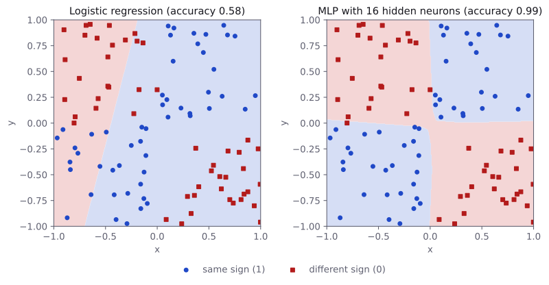
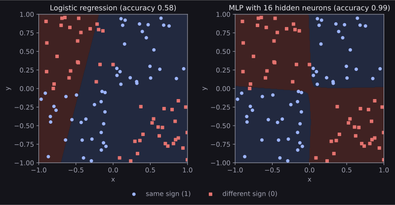
Each hidden neuron with ReLU contributes one bend, and the output layer adds the bends together. With 16 bends to work with, the network can trace the quarters. If we shrink the hidden layer to 2 neurons (nn.Linear(2, 2) and nn.Linear(2, 1)), the test accuracy drops to 0.85: too few bends. If we keep 16 neurons but delete the nn.ReLU() line, it drops to 0.59, no better than logistic regression, exactly as the collapse argument above predicts. Try both yourself.
The same MLP as a class
nn.Sequential is perfect when data simply flows through the layers in order. When a model needs more control, for example two inputs or a skip from one layer to a later one, we write it as a class that inherits from nn.Module, as in Classes and Inheritance. Here is the MLP from the example written that way:
class SignNet(nn.Module):
    def __init__(self, hidden_size):
        super().__init__()
        self.hidden = nn.Linear(2, hidden_size)
        self.activation = nn.ReLU()
        self.output = nn.Linear(hidden_size, 1)

    def forward(self, x):
        x = self.hidden(x)        # (batch, 2) -> (batch, hidden_size)
        x = self.activation(x)
        return self.output(x)     # (batch, hidden_size) -> (batch, 1)

net = SignNet(hidden_size=16)
net(test_x).shapetorch.Size([100, 1])__init__ creates the layers and stores them as attributes, and forward says how an input flows through them. Both versions train with exactly the same loop. You will meet both styles in PyTorch code, so it is worth being able to read each.
How big should the network be?
There is no formula, but a few rules of thumb cover most tabular tasks:
- Start small: one or two hidden layers with 32 to 256 neurons each is a reasonable first try.
- Width and depth trade off: a wider layer can make more bends at once; more layers can combine bends into more complicated shapes. For tabular data, going beyond three or four hidden layers often adds little.
- Bigger is not automatically better: more parameters also means more ability to memorise the training set. If the training loss keeps falling while the validation loss rises, the model is overfitting.
OptionalThe universal approximation theorem
The universal approximation theorem says that an MLP with a single hidden layer and a suitable nonlinear activation can approximate any continuous function on a bounded region as closely as you like, provided the hidden layer is wide enough.
It is a reassuring result, but it says nothing about how many neurons you need (possibly an enormous number), nor whether gradient descent will actually find the right weights, nor whether the result will generalise to new data. In practice, a deeper network can often do the same job with far fewer parameters than a single very wide layer. Chapter 4 of Nielsen's book gives a visual proof if you are curious. You do not need this theorem for anything in this guide.
Common mistakes
These are the mistakes that come up most often when building a first MLP. The messages are exactly what PyTorch prints.
| Mistake | What you see | Fix |
|---|---|---|
The first layer's input size does not match the number of features, e.g. nn.Linear(3, 1) on data with 2 features |
RuntimeError: mat1 and mat2 shapes cannot be multiplied (4x2 and 3x1) |
Set in_features to X.shape[1]. |
Output shape (300, 1) compared with labels of shape (300,) |
ValueError: Target size (torch.Size([300])) must be the same as input size (torch.Size([300, 1])) |
.squeeze(1) the scores, or reshape the labels. |
Forgetting super().__init__() in a class |
AttributeError: cannot assign module before Module.__init__() call |
Call it first in __init__. |
| No activation between the linear layers | No error, but the model can only draw straight boundaries | Put nn.ReLU() (or another activation) between layers. |
| An activation such as ReLU after the last layer | No error, but the scores can never be negative, so the model cannot say "confidently class 0" | Leave the output layer without an activation; the loss handles it. |
How to practise
There is no MLP section on the practice sites we use (CodeChef, CS50 and HackerRank), so practise with the course material and with your own experiments:
- Do the exercises at the end of chapter 1 of Nielsen's book and of the d2l MLP section.
- On the TensorFlow Playground, pick the XOR-like dataset (the one with four coloured quarters) and find the smallest network that separates it.
- Take the sign-pattern example above and change one thing at a time: the number of hidden neurons, the number of layers, the learning rate. Predict what will happen before you run it.
Check yourself
What comes next
- Gradient Descent: how the update step moves the weights downhill on the loss.
- Backpropagation: how the gradients for every weight are computed in one backward pass.
- Activation Functions and Loss Functions: the two choices we treated as black boxes on this page.
Resources
| Source | Title | Why read it |
|---|---|---|
| 3Blue1Brown | But what is a neural network? (Deep learning, chapter 1) | Our recommended starting point: a visual explanation of neurons, layers, weights and biases. |
| Michael Nielsen | Neural Networks and Deep Learning, chapter 1 | A free book. Chapter 1 builds a network for handwritten digits, with the maths written out. |
| Dive into Deep Learning | Multilayer Perceptrons | A free textbook section with the matrix notation used on this page and PyTorch code. |
| Stanford CS231n | Neural Networks Part 1: Setting up the Architecture | Course notes on neurons, layers and counting parameters. |
| PyTorch | Build the Neural Network | The official tutorial for nn.Module, nn.Sequential and nn.Linear. |
| TensorFlow Playground | Neural network playground | Train a small network in your browser and watch it bend its decision boundary. No code needed. |
Finished this module? Mark it done.
Comments
Stuck on something, spotted a mistake, or found a resource that helped you? Tell us below.
Loading comments