5.5 Absolute and squared distances

In Module 5.2, optimization meant choosing an input that makes an objective as small or large as possible. This lesson is a direct application: several locations or readings are fixed, and we choose one centre $c$. Our objective is the total distance from $c$ to those observations, or the total of their squared distances. We seek the $c$ that makes that total smallest.

The choice of objective matters. Minimizing ordinary distance gives a median on a line; minimizing squared distance gives a mean. The first can choose a meeting point that minimizes total travel. The second appears when one constant prediction is chosen to minimize squared error. This is intermediate optimization using absolute value, averages, and derivatives. OpenStax's mean-and-median lesson gives the statistical background.

A basic idea: the penalty changes the centre

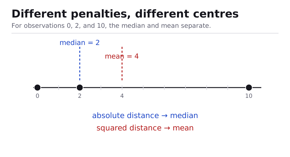
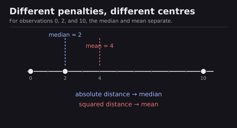
Take observations at $0,2,10$ on a number line. The decision is where to put $c$; the observations do not move. If we add ordinary distances, $c=2$ costs $|2-0|+|2-2|+|2-10|=10$, while $c=4$ costs $4+2+6=12$. Here $2$ is better. If we square each distance first, $c=2$ costs $4+0+64=68$, while $c=4$ costs $16+4+36=56$. Now $4$ is better.

The observation at $10$ is far from the others. Squaring its gap makes that large error especially costly, so the best squared-distance centre moves towards it. The best ordinary-distance centre stays at the middle observation. We will show below why these are global answers, not merely better than the two points compared here.

A quick tour of the two objectives

For fixed real observations $x_1,\ldots,x_n$, the variable we may choose is $c$. Two possible loss functions are

$$L_1(c)=\sum_{i=1}^n|c-x_i| \quad\text{or}\quad L_2(c)=\sum_{i=1}^n(c-x_i)^2.$$

For absolute distance $L_1$, imagine sliding $c$ a little to the right without crossing an observation. Each observation to its left becomes that much farther away; each observation to its right becomes that much closer. If more observations lie to the right, the total falls. If more lie to the left, it rises. The switch happens at a median. With an odd number of observations, the middle sorted value minimizes $L_1$; with an even number, every point between the two middle values gives the same minimum total.

For squared distance $L_2$, differentiation from Module 5.1 gives

$$L_2'(c)=2\sum_{i=1}^n(c-x_i)=2nc-2\sum_{i=1}^n x_i.$$

Set this slope to zero: $c=\sum_i x_i/n$, the mean. Also $L_2''(c)=2n>0$, so the loss bends upward and this is the global minimum. A distant observation has a larger effect because its squared error grows faster as the gap grows. For $0,2,10$, the mean is $4$, while the median is $2$.

If each observation has a positive weight $w_i$, use $\sum_iw_i|c-x_i|$ or $\sum_iw_i(c-x_i)^2$. The same reasoning gives a weighted median for absolute distance, with no more than half the total weight strictly to either side, and the weighted mean $\sum_iw_ix_i/\sum_iw_i$ for squared distance.

If a constraint restricts $c$ to an interval that excludes the median or mean, use Module 5.4's boundary check. For the observations $0,2,10$, requiring $c\ge5$ makes $c=5$ the best allowed choice for either loss.

The median result here is for distance on a line. For ordinary Euclidean distances to points in a plane, finding the geometric median needs a different method; this introductory module does not solve that general two-dimensional problem. For squared Euclidean distances in a plane, the coordinate-wise mean remains the minimizer.

Application 1: a meeting point on a road

Three teams are at road positions $1$, $2$, and $8$ kilometres. Where should they meet to minimize their total travel distance along the road?

1. Choose the objective. Total distance to meeting position $c$ is $|c-1|+|c-2|+|c-8|$.
2. Use the middle position. The sorted middle value is $2$. Just to its left, moving right reduces distance for two teams and increases it for one; just to its right, moving farther right increases distance for two teams and reduces it for one. The total is smallest at $c=2$ km.
3. Check. Total travel is $1+0+6=7$ km. At $c=4$, it would be $3+2+4=9$ km.

The farthest team does not by itself decide the best total-distance meeting point.

Application 2: one constant sensor estimate

Readings are $2$, $4$, $9$, and $11$ units. Choose one constant estimate $c$ that minimizes total squared error.

1. Write the objective. $L(c)=(c-2)^2+(c-4)^2+(c-9)^2+(c-11)^2$.
2. Find the minimum. $L'(c)=2[(c-2)+(c-4)+(c-9)+(c-11)]=8c-52$. Setting it to zero gives $c=6.5$ units, the mean $(2+4+9+11)/4$.
3. Check the loss. $L''(c)=8>0$, so this is a minimum. The squared errors are $20.25$, $6.25$, $6.25$, and $20.25$, totalling $53$.

The squared penalty makes larger errors count much more than small errors.