11.6 Row and column normalisation

Module 11.5 used a matrix whose rows each sum to $1$. Why? Each row describes all destinations for one current state, so the fractions leaving that state must account for its whole population or probability. Sometimes a question gives weights instead of probabilities, or a table appears to lose mass. Normalisation and conservation checks tell us what the numbers mean before we iterate them.

This is intermediate matrix work. Review transition matrices and matrix multiplication; MIT's Markov-chain notes develop stochastic matrices in greater depth. The central question here is simple: what enters, what leaves, and what is included in the state?

A basic idea: divide each source row by its total

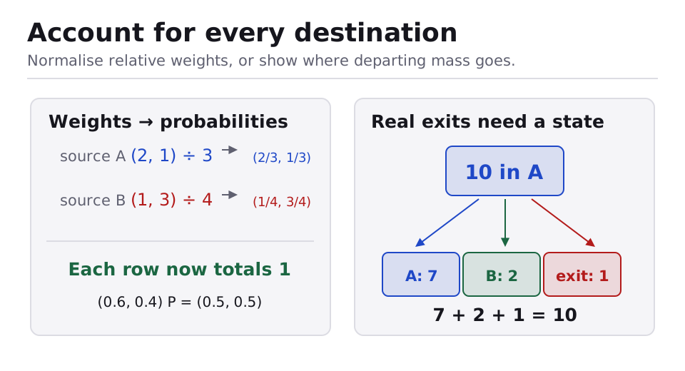
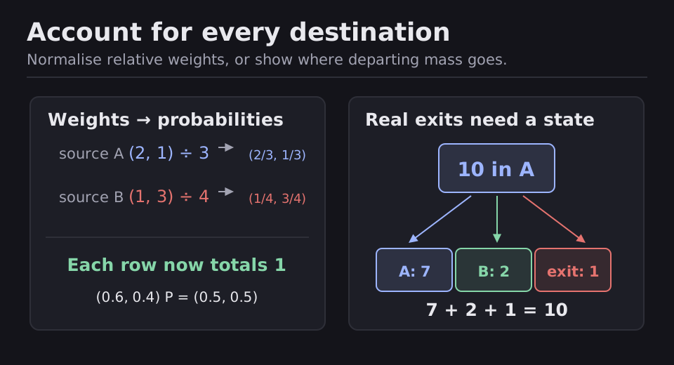
Suppose a table of nonnegative weights is $W=\begin{bmatrix}2&1\\1&3\end{bmatrix}$, with rows representing the current state and columns the destination. The first source row totals $3$, the second totals $4$. If these weights mean relative chances, divide within each row:

$$P=\begin{bmatrix}2/3&1/3\\1/4&3/4\end{bmatrix}.$$

Each row now sums to $1$. For a starting probability row $s_0=(0.6,0.4)$, the next distribution is $s_1=s_0P=(0.5,0.5)$. We redistributed all the probability; none disappeared.

A quick tour of sums and conservation

For a nonnegative weight matrix $W$, row normalisation uses $P_{ij}=W_{ij}/\sum_j W_{ij}$, provided that row total is positive. Then each row of $P$ sums to $1$, and a row-vector distribution updates by $s_{t+1}=s_tP$. A zero row cannot be divided by its sum; the model must specify what happens there, such as staying put or entering an exit state.

Why is total probability conserved? Every old state's mass is split across destinations whose shares total $1$. Algebraically, with $\mathbf1$ the column of all ones, $P\mathbf1=\mathbf1$, so $(s_tP)\mathbf1=s_t\mathbf1$. This is the total before and after the update. The same argument works for counts if the fractions describe movement without creation or loss.

For column vectors, put source states in the columns. The corresponding matrix is $C=P^{\mathsf T}$, whose columns sum to $1$, and $x_{t+1}=Cx_t$. If a raw weight table already uses columns as sources, divide each nonzero column by its column total. Check which index means “from” before normalising; a row-stochastic matrix applied to a column vector generally does not preserve the total.

If the listed states exclude an exit, the displayed total may fall. That can be a correct model of loss from the tracked system. Normalising it to sum to $1$ would change the model into a conditional one: where the remaining mass goes given that it did not exit. Include an explicit exit state when you need to track all mass.

Application 1: relative movement weights

The source-to-destination weights are $W=\begin{bmatrix}2&1\\1&3\end{bmatrix}$. Start with probabilities $(0.6,0.4)$. Find the next distribution.

1. Row totals are $3$ and $4$, so $P=\begin{bmatrix}2/3&1/3\\1/4&3/4\end{bmatrix}$.
2. The next first-state probability is $0.6(2/3)+0.4(1/4)=0.5$; the second is $0.6(1/3)+0.4(3/4)=0.5$.
3. Both entries are nonnegative and total $1$, as a probability distribution must.

Application 2: a real exit

Suppose an incomplete table lists only two destinations, with rows $(0.7,0.2)$ and $(0.1,0.6)$. Ten items all start in state $A$. What happens after one step?

1. The first row totals $0.9$, so $10$ items become $7$ in $A$ and $2$ in $B$; one item leaves the two tracked states. Do not silently divide $0.7$ and $0.2$ by $0.9$ if departure is real.
2. Add an exit state $E$ with the missing shares. One complete matrix is $P=\begin{bmatrix}0.7&0.2&0.1\\0.1&0.6&0.3\\0&0&1\end{bmatrix}$, in the order $(A,B,E)$.
3. $(10,0,0)P=(7,2,1)$, whose total is still $10$. The exit state makes the loss from the first two states visible.