5.3 Convex and quadratic optimisation

Two graphs can both have a flat point yet behave differently. A convex graph bends upward like a bowl; a concave graph bends downward like a cap. For a quadratic, this shape tells us whether its vertex is a global minimum or maximum, not merely a possible turning point.

This is intermediate calculus and algebra. Review quadratic equations, quadratic graphs, and maxima and minima. OpenStax's graph-shape lesson develops the derivative connection.

A basic idea: watch the slopes

On $f(x)=x^2$, slopes rise as $x$ moves right: negative, then zero, then positive. The graph bends upward and $x=0$ gives its lowest value. On $g(x)=-x^2$, slopes fall as $x$ moves right: positive, then zero, then negative. That graph bends downward and $x=0$ gives its highest value.

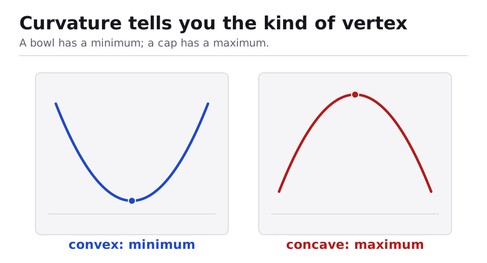
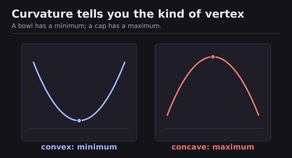
A quick tour of curvature and quadratics

The second derivative $f''(x)$ describes how the slope $f'(x)$ changes. On an interval, $f''(x)>0$ means slopes increase and the graph is concave up; $f''(x)<0$ means slopes decrease and it is concave down. A point where the curvature changes sign is an inflection point. A zero second derivative alone does not prove that a change occurs.

For $Q(x)=ax^2+bx+c$ with $a\ne0$,

$$Q'(x)=2ax+b,\qquad Q''(x)=2a,\qquad h=-\frac{b}{2a}.$$

The vertex is at $(h,Q(h))$. Completing the square gives $Q(x)=a(x-h)^2+Q(h)$. Since $(x-h)^2\ge0$, $a>0$ makes $Q(h)$ the global minimum over all real $x$; $a<0$ makes it the global maximum. This proves the result without relying only on a sketch.

For a general convex differentiable function on an interval, a point with $f'(x)=0$ is a global minimum on that interval. The analogous statement holds for a concave function and a maximum. Constraints can remove that point from the allowed domain, so still check the feasible set.

Application 1: choose a constant prediction

A constant prediction $c$ is compared with values $1,3,8$ using total squared error $L(c)=(c-1)^2+(c-3)^2+(c-8)^2$. Which $c$ minimizes it?

1. Differentiate. $L'(c)=2(c-1)+2(c-3)+2(c-8)=6c-24$.
2. Find the flat point. $L'(c)=0$ gives $c=4$.
3. Confirm the shape. $L''(c)=6>0$, so this is the global minimum. The error is $L(4)=9+1+16=26$.

The minimizing constant is the mean of the three values. Module 5.5 explains why this happens more generally.

Application 2: a price and demand model

A simplified model says selling at price $p$ gives demand $20-p$ units, for $0\le p\le20$. Revenue is $R(p)=p(20-p)$. Which price maximizes revenue?

1. Expand and differentiate. $R(p)=-p^2+20p$, so $R'(p)=20-2p$.
2. Find the vertex. $R'(p)=0$ gives $p=10$.
3. Confirm and interpret. $R''(p)=-2<0$, so the cap peaks there. Revenue is $R(10)=100$ model units; at prices $0$ and $20$ it is $0$.

The price $10$ is inside the allowed range, so it is also the constrained maximum here.